[1]:
%run ../initscript.py
HTML("""
<div id="popup" style="padding-bottom:5px; display:none;">
<div>Enter Password:</div>
<input id="password" type="password"/>
<button onclick="done()" style="border-radius: 12px;">Submit</button>
</div>
<button onclick="unlock()" style="border-radius: 12px;">Unclock</button>
<a href="#" onclick="code_toggle(this); return false;">show code</a>
""")
[1]:
[2]:
%run ../../notebooks/loadtsfuncs.py
%matplotlib inline
toggle()
[2]:
Stationarity and Forecastability
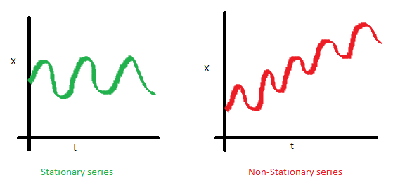
A time series is stationary if the values of the series is not a function of time. Therefore, A stationary time series has constant mean and variance. More importantly, the correlation of the series with its previous values (lags) is also constant. The correlation is called Autocorrelation.
The mean of the series should not be a function of time. The red graph below is not stationary because the mean increases over time.
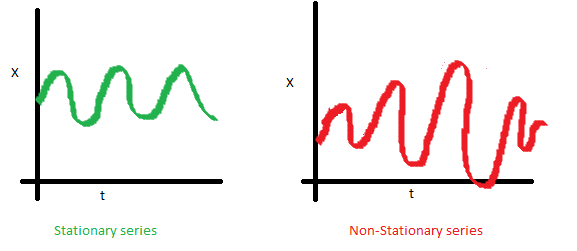
The variance of the series should not be a function of time. This property is known as homoscedasticity. Notice in the red graph the varying spread of data over time.
Finally, the covariance of the \(i\)th time and the \((i + m)\)th time should not be a function of time. In the following graph, we notice the spread becomes closer as the time increases. Hence, the covariance is not constant with time for the ‘red series’. 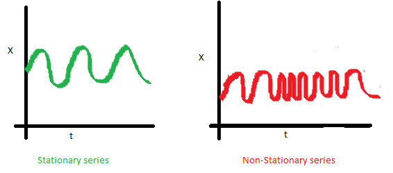
For example, white noise is a stationary series. However, random walk is always non-stationary because of its variance depends on time.
How to Make a Time Series Stationary?
It is possible to make nearly any time series stationary by applying a suitable transformation. The first step in the forecasting process is typically to do some transformation to convert a non-stationary series to stationary. The transformation includes 1. Differencing the Series (once or more) 2. Take the log of the series 3. Take the nth root of the series 4. Combination of the above
The most common and convenient method to stationarize a series is by differencing. Let \(Y_t\) be the value at time \(t\), the fist difference of \(Y\) is \(Y_t - Y_{t-1}\), i.e., subtracting the next value by the current value. If the first difference does not make a series stationary, we can apply the second differencing, and so on.
[3]:
Y = [1, 5, 8, 3, 15, 20]
print('Y = {}\nFirst differencing is {}, Second differencing is {}'.format(Y, np.diff(Y,1), np.diff(Y,2)))
toggle()
Y = [1, 5, 8, 3, 15, 20]
First differencing is [ 4 3 -5 12 5], Second differencing is [-1 -8 17 -7]
[3]:
Why does a Stationary Series Matter?
Most statistical forecasting methods are designed to work on a stationary time series.
Forecasting a stationary series is relatively easy and the forecasts are more reliable.
An important reason is, autoregressive forecasting models are essentially linear regression models that utilize the lag(s) of the series itself as predictors.
We know that linear regression works best if the predictors (\(X\) variables) are not correlated against each other. So, stationarizing the series solves this problem since it removes any persistent autocorrelation, thereby making the predictors(lags of the series) in the forecasting models nearly independent.
Test for Stationarity
The most commonly used is the Augmented Dickey Fuller (ADF) test, where the null hypothesis is the time series possesses a unit root and is non-stationary. So, if the P-Value in ADH test is less than the significance level (for example 5%), we reject the null hypothesis.
The KPSS test, on the other hand, is used to test for trend stationarity. If \(Y_t\) is a trend-stationary process, then
where: - \(\mu_t\) is a deterministic mean trend, - \(e_t\) is a stationary stochastic process with mean zero.
For the KPSS test, the null hypothesis and the P-Value interpretation is just the opposite of ADH test. The below code implements these two tests using statsmodels package in python.
[4]:
stationarity_test(df_house.sales, title='House Sales')
Test on House Sales:
ADF Statistic : -1.72092
p-value : 0.42037
Critial Values :
1.0% : -3.45375
5.0% : -2.87184
10.0% : -2.57226
H0: The time series is non-stationary
We do not reject the null hypothesis.
KPSS Statistic : 0.50769
p-value : 0.03993
Critial Values :
10.0% : 0.34700
5.0% : 0.46300
2.5% : 0.57400
1.0% : 0.73900
H0: The time series is stationary
We reject the null hypothesis at 5% level.
[5]:
stationarity_test(df_drink.sales, title='Drink Sales')
Test on Drink Sales:
ADF Statistic : -0.83875
p-value : 0.80747
Critial Values :
1.0% : -3.55527
5.0% : -2.91573
10.0% : -2.59567
H0: The time series is non-stationary
We do not reject the null hypothesis.
KPSS Statistic : 0.62519
p-value : 0.02035
Critial Values :
10.0% : 0.34700
5.0% : 0.46300
2.5% : 0.57400
1.0% : 0.73900
H0: The time series is stationary
We reject the null hypothesis at 5% level.
Estimate the Forecastability
The more regular and repeatable patterns a time series has, the easier it is to forecast.
The Approximate Entropy can be used to quantify the regularity and unpredictability of fluctuations in a time series. The higher the approximate entropy, the more difficult it is to forecast it.
A better alternate is the Sample Entropy. Sample Entropy is similar to approximate entropy but is more consistent in estimating the complexity even for smaller time series. For example, a random time series with fewer data points can have a lower approximate entropy than a more regular time series, whereas, a longer random time series will have a higher approximate entropy.
[6]:
# https://en.wikipedia.org/wiki/Approximate_entropy
rand_small = np.random.randint(0, 100, size=50)
rand_big = np.random.randint(0, 100, size=150)
def ApproxEntropy(U, m, r):
"""Compute Aproximate entropy"""
def _maxdist(x_i, x_j):
return max([abs(ua - va) for ua, va in zip(x_i, x_j)])
def _phi(m):
x = [[U[j] for j in range(i, i + m - 1 + 1)] for i in range(N - m + 1)]
C = [len([1 for x_j in x if _maxdist(x_i, x_j) <= r]) / (N - m + 1.0) for x_i in x]
return (N - m + 1.0)**(-1) * sum(np.log(C))
N = len(U)
return abs(_phi(m+1) - _phi(m))
print("House data\t: {:.2f}".format(ApproxEntropy(df_house.sales, m=2, r=0.2*np.std(df_house.sales))))
print("Drink data\t: {:.2f}".format(ApproxEntropy(df_drink.sales, m=2, r=0.2*np.std(df_drink.sales))))
print("small size random integer\t: {:.2f}".format(ApproxEntropy(rand_small, m=2, r=0.2*np.std(rand_small))))
print("large size random integer\t: {:.2f}".format(ApproxEntropy(rand_big, m=2, r=0.2*np.std(rand_big))))
toggle()
House data : 0.53
Drink data : 0.55
small size random integer : 0.38
large size random integer : 0.70
[6]:
The random data should be more difficult to forecast. However, small size data can have small approximate entropy.
[7]:
# https://en.wikipedia.org/wiki/Sample_entropy
def SampleEntropy(U, m, r):
"""Compute Sample entropy"""
def _maxdist(x_i, x_j):
return max([abs(ua - va) for ua, va in zip(x_i, x_j)])
def _phi(m):
x = [[U[j] for j in range(i, i + m - 1 + 1)] for i in range(N - m + 1)]
C = [len([1 for j in range(len(x)) if i != j and _maxdist(x[i], x[j]) <= r]) for i in range(len(x))]
return sum(C)
N = len(U)
return -np.log(_phi(m+1) / _phi(m))
print("House sales data\t: {:.2f}".format(SampleEntropy(df_house.sales, m=2, r=0.2*np.std(df_house.sales))))
print("Drink sales data\t: {:.2f}".format(SampleEntropy(df_drink.sales, m=2, r=0.2*np.std(df_drink.sales))))
print("small size random integer\t: {:.2f}".format(SampleEntropy(rand_small, m=2, r=0.2*np.std(rand_small))))
print("large size random integer\t: {:.2f}".format(SampleEntropy(rand_big, m=2, r=0.2*np.std(rand_big))))
toggle()
House sales data : 0.44
Drink sales data : 1.03
small size random integer : 1.66
large size random integer : 2.03
[7]:
Sample Entropy handles the problem nicely and shows that random data is difficult to forecast.
Granger Causality Test
Granger causality test is used to determine if one time series will be useful to forecast another. The idea is that if \(X\) causes \(Y\), then the forecast of \(Y\) based on previous values of \(Y\) AND the previous values of \(X\) should outperform the forecast of \(Y\) based on previous values of \(Y\) alone.
Therefore, Granger causality should not be used to test if a lag of \(Y\) causes \(Y\). Instead, it is generally used on exogenous (not \(Y\) lag) variables only.
The null hypothesis is: the series in the second column does not Granger cause the series in the first. If the P-Values are less than a significance level (for example 5%) then you reject the null hypothesis and conclude that the said lag of \(X\) is indeed useful. The second argument maxlag says till how many lags of \(Y\) should be included in the test.
[8]:
# https://en.wikipedia.org/wiki/Granger_causality
from statsmodels.tsa.stattools import grangercausalitytests
df_house['m'] = df_house.index.month
# The values are in the first column and the predictor (X) is in the second column.
_ = grangercausalitytests(df_house[['sales', 'm']], maxlag=2)
toggle()
Granger Causality
number of lags (no zero) 1
ssr based F test: F=0.1690 , p=0.6813 , df_denom=290, df_num=1
ssr based chi2 test: chi2=0.1708 , p=0.6794 , df=1
likelihood ratio test: chi2=0.1707 , p=0.6795 , df=1
parameter F test: F=0.1690 , p=0.6813 , df_denom=290, df_num=1
Granger Causality
number of lags (no zero) 2
ssr based F test: F=0.6936 , p=0.5006 , df_denom=287, df_num=2
ssr based chi2 test: chi2=1.4115 , p=0.4938 , df=2
likelihood ratio test: chi2=1.4081 , p=0.4946 , df=2
parameter F test: F=0.6936 , p=0.5006 , df_denom=287, df_num=2
[8]:
[9]:
df_drink['q'] = df_drink.index.quarter
_ = grangercausalitytests(df_drink[['sales', 'q']], maxlag=2)
toggle()
Granger Causality
number of lags (no zero) 1
ssr based F test: F=74.3208 , p=0.0000 , df_denom=60, df_num=1
ssr based chi2 test: chi2=78.0368 , p=0.0000 , df=1
likelihood ratio test: chi2=50.7708 , p=0.0000 , df=1
parameter F test: F=74.3208 , p=0.0000 , df_denom=60, df_num=1
Granger Causality
number of lags (no zero) 2
ssr based F test: F=108.5323, p=0.0000 , df_denom=57, df_num=2
ssr based chi2 test: chi2=236.1053, p=0.0000 , df=2
likelihood ratio test: chi2=97.3594 , p=0.0000 , df=2
parameter F test: F=108.5323, p=0.0000 , df_denom=57, df_num=2
[9]:
For the drink sales data, the P-Values are 0 for all tests. So the quarter indeed can be used to forecast drink sales.