%run ../initscript.py
HTML("""
<div id="popup" style="padding-bottom:5px; display:none;">
    <div>Enter Password:</div>
    <input id="password" type="password"/>
    <button onclick="done()" style="border-radius: 12px;">Submit</button>
</div>
<button onclick="unlock()" style="border-radius: 12px;">Unclock</button>
<a href="#" onclick="code_toggle(this); return false;">show code</a>
""")

Enter Password:

Submit

Unclock show code

%run ../../notebooks/loadtsfuncs.py
%matplotlib inline
toggle()

show code

Exponential Smoothing Forecasts

Simple Exponential Smoothing

The simple exponential smoothing method is defined by the following two equations, where

• \(L_t\), called the level of the series at time \(t\), is not observable but can only be estimated. Essentially, it is an estimate of where the series would be at time \(t\) if there were no random noise.

• \(F_{t+k}\) is the forecast of \(Y_{t+k}\) made at time \(t\).

\begin{align} L_t &= \alpha Y_t + (1-\alpha) L_{t-1} \tag{1}\\ F_{t+k} &= L_t \nonumber \end{align}

The level \(\alpha \in [0,1]\). If you want the method to react quickly to movements in the series, you should choose a large \(\alpha\); otherwise a small \(\alpha\).

• If \(\alpha\) is close to 0, observations from the distant past continue to have a large influence on the next forecast. This means that the graph of the forecasts will be relatively smooth.

• If \(\alpha\) is close to 1, only very recent observations have much influence on the next forecast. In this case, forecasts react quickly to sudden changes in the series.

Simple exponential smoothing offers “flat” forecasts. That is, all forecasts take the same value, equal to the last level component. Remember that these forecasts will only be suitable if the time series has no trend or seasonal component.

Why exponential smoothing?

Note that

\begin{align} L_{t-1} &= \alpha Y_{t-1} + (1-\alpha) L_{t-2} \tag{2} \\ \end{align}

By substituting equation (2) into equation (1), we get

\begin{align*} L_{t} &= \alpha Y_{t-1} + (1-\alpha) \big( \alpha Y_{t-1} + (1-\alpha) L_{t-2} \big) \\ &= \alpha Y_{t-1} + \alpha(1-\alpha) Y_{t-1} + (1-\alpha)^2 L_{t-2} \end{align*}

If we substitute recursively into the equation (1), we obtain

\begin{align*} L_{t} &= \alpha Y_{t-1} + \alpha(1-\alpha) Y_{t-1} + \alpha(1-\alpha)^2 Y_{t-2} + \alpha(1-\alpha)^3 Y_{t-3} + \cdots \end{align*}

where exponentially decaying weights are assigned to historical data.

widgets.interact_manual.opts['manual_name'] = 'Run Forecast'
interact_manual(ses_forecast,
         forecasts=widgets.BoundedIntText(value=12, min=1, description='Forecasts:', disabled=False),
         holdouts=widgets.BoundedIntText(value=0, min=0, description='Holdouts:', disabled=False),
         level=widgets.BoundedFloatText(value=0.2, min=0, max=1, step=0.05, description='Level:', disabled=False),
         optimized=widgets.Checkbox(value=False, description='Optimize Parameters', disabled=False));

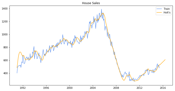
Holt’s Model for Trend

Holt extended simple exponential smoothing to allow the forecasting of data with a trend. This method involves a forecast equation and two smoothing equations where one for the level and one for the trend.

Besides the smoothing constant \(\alpha\) for the level, Holt’s requires a new smoothing constant \(\beta\) for the trend to control how quickly the method reacts to observed changes in the trend.

• If \(\beta\) is small, the method reacts slowly,

• If \(\beta\) is large, the method reacts more quickly.

Some practitioners suggest using a small value of \(\alpha\) (such as 0.1 to 0.2) and setting \(\beta = \alpha\). Others suggest using an optimization option to select the optimal smoothing constant.

from statsmodels.tsa.holtwinters import Holt

# df_house.index.freq = 'MS'
plt.figure(figsize=(12, 6))
train = df_house.iloc[:, 0]
train.index = pd.DatetimeIndex(train.index.values, freq=train.index.inferred_freq)
model = Holt(train).fit(smoothing_level=0.2, smoothing_slope=0.2, optimized=False)
pred = model.predict(start=train.index[0], end=train.index[-1] + 12*train.index.freq)

plt.plot(train.index, train, label='Train', c='cornflowerblue')
plt.plot(pred.index, pred, label='Holt\'s', c='orange')
plt.legend(loc='best')
plt.title('House Sales')
plt.show()

toggle()

show code

Damped Trend Methods

The forecasts generated by Holt’s linear method display a constant trend (increasing or decreasing) indefinitely into the future. Empirical evidence indicates that these methods tend to over-forecast, especially for longer forecast horizons. Motivated by this observation, Gardner & McKenzie introduced a parameter that “dampens” the trend to a flat line some time in the future. Methods that include a damped trend have proven to be very successful, and are arguably the most popular individual methods when forecasts are required automatically for many series.

Holt(train, exponential=False, damped=True).fit(...,damping_slope=)

In practice, the damping factor is rarely less than 0.8 as the damping has a very strong effect for smaller values. The damping factor close to 1 will mean that a damped model is not able to be distinguished from a non-damped model. For these reasons, we usually restrict the damping factor to a minimum of 0.8 and a maximum of 0.98.

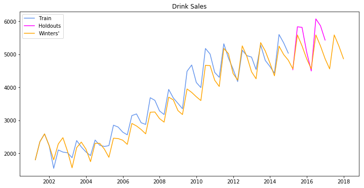
Winters’ Exponential Smoothing Model

The Holt-Winters seasonal method comprises the forecast equation and three smoothing equations: one for the level, one for the trend, and one for the seasonal component.

We use \(m\) to denote the frequency of the seasonality, i.e., the number of seasons in a year. For example, for quarterly data \(m = 4\), and for monthly data \(m=12\). There are two variations to this method that differ in the nature of the seasonal component.

• The additive method is preferred when the seasonal variations are roughly constant through the series. With the additive method, the seasonal component is expressed in absolute terms in the scale of the observed series, and in the level equation the series is seasonally adjusted by subtracting the seasonal component. Within each year, the seasonal component will add up to approximately zero.

• The multiplicative method is preferred when the seasonal variations are changing proportional to the level of the series. With the multiplicative method, the seasonal component is expressed in relative terms (percentages), and the series is seasonally adjusted by dividing through by the seasonal component. Within each year, the seasonal component will sum up to approximately \(m\) (average to 1).

from statsmodels.tsa.holtwinters import ExponentialSmoothing

plt.figure(figsize=(12, 6))
train, test = df_drink.iloc[:-8, 0], df_drink.iloc[-8:,0]
train.index = pd.DatetimeIndex(train.index.values, freq=train.index.inferred_freq)

model = ExponentialSmoothing(train, seasonal='mul', seasonal_periods=4).fit(smoothing_level=0.2,
                                        smoothing_slope=0.2,
                                        smoothing_seasonal=0.4,
                                        optimized=False)
pred = model.predict(start=train.index[0], end=test.index[-1] + 4*train.index.freq)

plt.plot(train.index, train, label='Train', c='cornflowerblue')
plt.plot(test.index, test, label='Holdouts', c='fuchsia')
plt.plot(pred.index, pred, label='Winters\'', c='orange')
plt.legend(loc='best')
plt.title('Drink Sales')
plt.show()

toggle()

show code

Holt-Winters’ damped method

Damping is possible with both additive and multiplicative Holt-Winters’ methods. A method that often provides accurate and robust forecasts for seasonal data is the Holt-Winters method with a damped trend and multiplicative seasonality