[1]:
%run ../initscript.py
HTML("""
<div id="popup" style="padding-bottom:5px; display:none;">
<div>Enter Password:</div>
<input id="password" type="password"/>
<button onclick="done()" style="border-radius: 12px;">Submit</button>
</div>
<button onclick="unlock()" style="border-radius: 12px;">Unclock</button>
<a href="#" onclick="code_toggle(this); return false;">show code</a>
""")
[1]:
[2]:
%run ../../notebooks/loadtsfuncs.py
%matplotlib inline
toggle()
[2]:
ARIMA Models
ARIMA is an acronym that stands for AutoRegressive Integrated Moving Average. It is a forecasting algorithm based on the idea that the information in the past values of the time series (i.e. its own lags and the lagged forecast errors) can alone be used to predict the future values.
Any non-seasonal time series that exhibits patterns and is not a random white noise can be modeled with ARIMA models.
The acronym ARIMA is descriptive, capturing the key aspects of the model itself. Briefly, they are:
AR: Autoregression. A model that uses the dependent relationship between an observation and some number of lagged observations. An autoregressive model of order \(p\) (AR(p)) can be written as
I: Integrated. The use of differencing of raw observations (e.g. subtracting an observation from an observation at the previous time step) in order to make the time series stationary.
MA: Moving Average. A model that uses the dependency between an observation and a residual error from a moving average model applied to lagged observations. An moving average model of order \(q\) (MA(q)) can be written as
Each of these components are explicitly specified in the model as a parameter. A standard notation is used of ARIMA(p,d,q) where the parameters are substituted with integer values to quickly indicate the specific ARIMA model being used. The parameters of the ARIMA model are defined as follows:
\(d\) is the number of differencing required to make the time series stationary
\(p\) is the number of lag observations included in the model, i.e., the order of the AR term
\(q\) is The size of the moving average window, i.e., the order of the MA term
The ARIMA(p,d,q) model can be written as
\begin{equation} Y^\prime_{t} = c + \phi_{1}Y^\prime_{t-1} + \cdots + \phi_{p}Y^\prime_{t-p} + \theta_{1}e_{t-1} + \cdots + \theta_{q}e_{t-q} + e_{t}, \end{equation}
where \(Y^\prime_{t}\) is the differenced series (it may have been differenced more than once). The ARIMA\((p,d,q)\) model in words:
predicted \(Y_t\) = Constant + Linear combination Lags of \(Y\) (upto \(p\) lags) + Linear Combination of Lagged forecast errors (upto \(q\) lags)
The objective, therefore, is to identify the values of p, d and q. A value of 0 can be used for a parameter, which indicates to not use that element of the model. This way, the ARIMA model can be configured to perform the function of an ARMA model, and even a simple AR, I, or MA model.
How to make a series stationary?
The most common approach is to difference it. That is, subtract the previous value from the current value. Sometimes, depending on the complexity of the series, more than one differencing may be needed.
The value of \(d\), therefore, is the minimum number of differencing needed to make the series stationary. And if the time series is already stationary, then \(d = 0\).
Why make the time series stationary?
Because, term “Auto Regressive” in ARIMA means it is a linear regression model that uses its own lags as predictors. Linear regression models work best when the predictors are not correlated and are independent of each other. So we take differences to remove trend and seasonal structures that negatively affect the regression model.
Identify the Order of Differencing
The right order of differencing is the minimum differencing required to get a near-stationary series which roams around a defined mean and the ACF plot reaches to zero fairly quick. If the autocorrelations are positive for many number of lags (10 or more), then the series needs further differencing. On the other hand, if the lag 1 autocorrelation itself is too negative, then the series is probably over-differenced. If we can’t really decide between different orders of differencing, then go with the order that gives the least standard deviation in the differenced series.
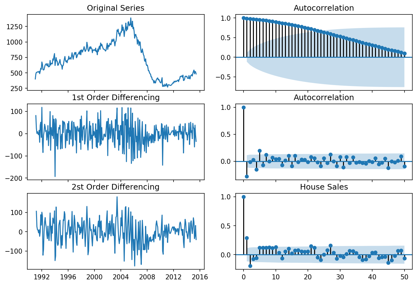
[3]:
differencing(df_house, 'sales', title='House Sales')
Standard deviation original series: 279.720
Standard deviation 1st differencing: 48.344
Standard deviation 2st differencing: 57.802
[4]:
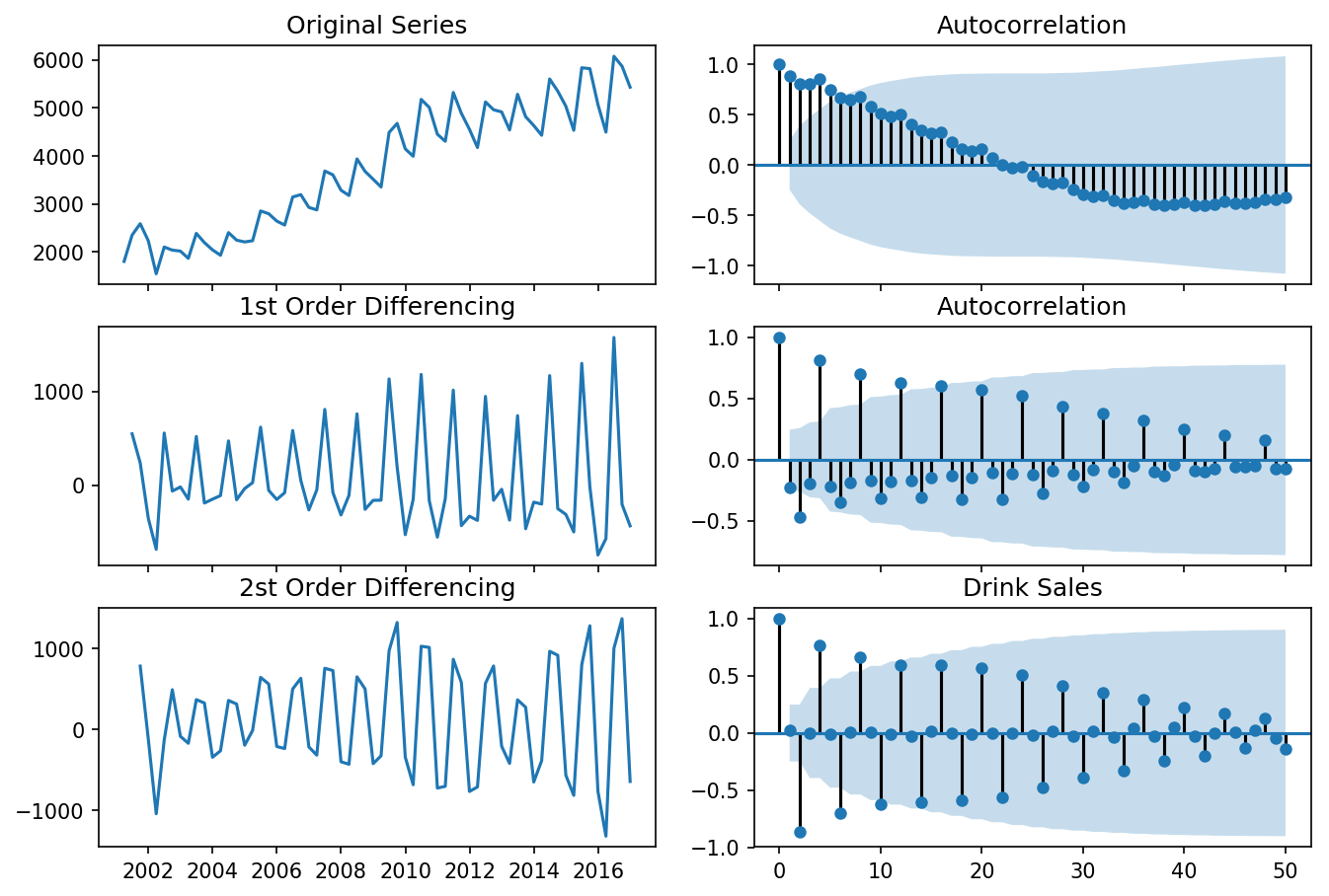
differencing(df_drink, 'sales', title='Drink Sales')
Standard deviation original series: 1283.446
Standard deviation 1st differencing: 532.296
Standard deviation 2st differencing: 661.759
Recall that ADF test shows that the house sales data is not stationary. On looking at the autocorrelation plot for the first differencing the lag goes into the negative zone, which indicates that the series might have been over differenced. We tentatively fix the order of differencing as \(d=1\) even though the series is a bit overdifferenced.
Identify the Order of the MA and AR Terms
If the ACF of the differenced series displays a sharp cutoff and/or the lag-1 autocorrelation is negative - i.e., if the series appears slightly “overdifferenced” - then consider adding an MA term to the model. The lag at which the ACF cuts off is the indicated number of MA terms.
If the PACF of the differenced series displays a sharp cutoff and/or the lag-1 autocorrelation is positive - i.e., if the series appears slightly “underdifferenced” - then consider adding an AR term to the model. The lag at which the PACF cuts off is the indicated number of AR terms.
[5]:
from statsmodels.graphics.tsaplots import plot_acf, plot_pacf
plt.rcParams.update({'figure.figsize':(9,3), 'figure.dpi':120})
fig, axes = plt.subplots(1, 2)
plot_acf(df_house.sales.diff().dropna(), lags=30, ax=axes[0])
plot_pacf(df_house.sales.diff().dropna(), lags=30, ax=axes[1])
plt.show()
toggle()
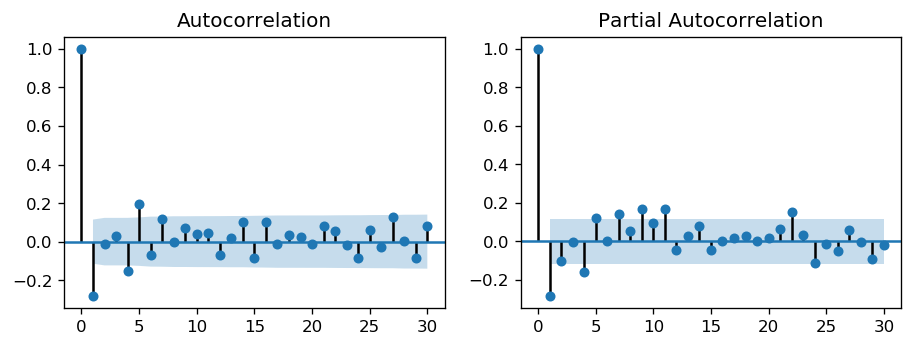
[5]:
The single negative spike at lag 1 in the ACF is an MA(1) signature, according to rule above. Thus, if we were to use 1 nonseasonal differences, we would also want to include an MA(1) term, yielding an ARIMA(0,1,1) model.
In most cases, the best model turns out a model that uses either only AR terms or only MA terms, although in some cases a “mixed” model with both AR and MA terms may provide the best fit to the data. However, care must be exercised when fitting mixed models. It is possible for an AR term and an MA term to cancel each other’s effects, even though both may appear significant in the model (as judged by the t-statistics of their coefficients).
[6]:
widgets.interact_manual.opts['manual_name'] = 'Run ARIMA'
interact_manual(arima_,
p=widgets.BoundedIntText(value=0, min=0, step=1, description='p:', disabled=False),
d=widgets.BoundedIntText(value=1, min=0, max=2, step=1, description='d:', disabled=False),
q=widgets.BoundedIntText(value=1, min=0, step=1, description='q:', disabled=False));
The table in the middle is the coefficients table where the values under coef are the weights of the respective terms. Ideally, we expect to have the P-Value in P>|z| column is less than 0.05 for the respective coef to be significant.
The setting dynamic=False in plot_predict uses the in-sample lagged values for prediction. The model gets trained up until the previous value to make the next prediction. This setting can make the fitted forecast and actuals look artificially good. Hence, we seem to have a decent ARIMA model. But is that the best? Can’t say that at this point because we haven’t actually forecasted into the future and compared the forecast with the actual performance. The real validation you need now is
the Out-of-Sample cross-validation.
Identify the Optimal ARIMA Model
We create the training and testing datasets by splitting the time series into two contiguous parts in approximately 75:25 ratio or a reasonable proportion based on time frequency of series.
[7]:
widgets.interact_manual.opts['manual_name'] = 'Run ARIMA'
interact_manual(arima_validation,
p=widgets.BoundedIntText(value=0, min=0, step=1, description='p:', disabled=False),
d=widgets.BoundedIntText(value=1, min=0, max=2, step=1, description='d:', disabled=False),
q=widgets.BoundedIntText(value=1, min=0, step=1, description='q:', disabled=False));
The model seems to give a directionally correct forecast and the actual observed values lie within the 95% confidence band.
A much more convenient approach is to use auto_arima() which searches multiple combinations of \(p,d,q\) parameters and chooses the best model. see auto_arima() manual for parameters settings.
[8]:
from statsmodels.tsa.arima_model import ARIMA
arima_house = pm.auto_arima(df_house.sales,
start_p=0, start_q=0,
test='adf', # use adftest to find optimal 'd'
max_p=4, max_q=4, # maximum p and q
m=12, # 12 for monthly data
d=None, # let model determine 'd' differencing
seasonal=False, # No Seasonality
#start_P=0, # order of the auto-regressive portion of the seasonal model
#D=0, # order of the seasonal differencing
#start_Q=0, # order of the moving-average portion of the seasonal model
trace=True,
error_action='ignore',
suppress_warnings=True,
stepwise=True)
display(arima_house.summary())
_ = arima_house.plot_diagnostics(figsize=(10,7));
toggle()
Fit ARIMA: order=(0, 1, 0); AIC=3108.202, BIC=3115.562, Fit time=0.003 seconds
Fit ARIMA: order=(1, 1, 0); AIC=3085.720, BIC=3096.761, Fit time=0.044 seconds
Fit ARIMA: order=(0, 1, 1); AIC=3082.268, BIC=3093.308, Fit time=0.032 seconds
Fit ARIMA: order=(1, 1, 1); AIC=3084.181, BIC=3098.901, Fit time=0.097 seconds
Fit ARIMA: order=(0, 1, 2); AIC=3084.182, BIC=3098.903, Fit time=0.050 seconds
Fit ARIMA: order=(1, 1, 2); AIC=3086.179, BIC=3104.580, Fit time=0.158 seconds
Total fit time: 0.402 seconds
| Dep. Variable: | D.y | No. Observations: | 293 |
|---|---|---|---|
| Model: | ARIMA(0, 1, 1) | Log Likelihood | -1538.134 |
| Method: | css-mle | S.D. of innovations | 46.084 |
| Date: | Thu, 16 May 2019 | AIC | 3082.268 |
| Time: | 15:00:10 | BIC | 3093.308 |
| Sample: | 1 | HQIC | 3086.690 |
| coef | std err | z | P>|z| | [0.025 | 0.975] | |
|---|---|---|---|---|---|---|
| const | 0.2164 | 1.823 | 0.119 | 0.906 | -3.356 | 3.789 |
| ma.L1.D.y | -0.3241 | 0.057 | -5.724 | 0.000 | -0.435 | -0.213 |
| Real | Imaginary | Modulus | Frequency | |
|---|---|---|---|---|
| MA.1 | 3.0859 | +0.0000j | 3.0859 | 0.0000 |
[8]:
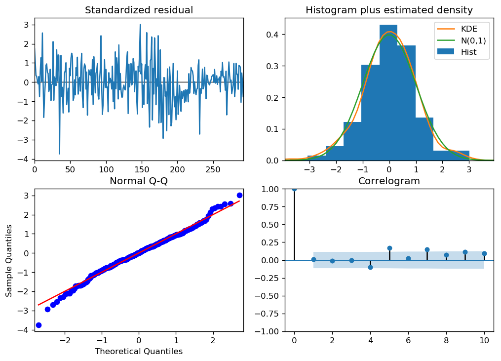
We can review the residual plots.
Standardized resitual: The residual errors seem to fluctuate around a mean of zero and have a uniform variance.
Histogram plus estimated density: The density plot suggests normal distribution with mean zero.
Normal Q-Q: All the dots should fall perfectly in line with the red line. Any significant deviations would imply the distribution is skewed.
Correlogram: The Correlogram (ACF plot) shows the residual errors are not autocorrelated. Any autocorrelation would imply that there is some pattern in the residual errors which are not explained in the model.
ARIMA Forecast
[9]:
# Forecast
n_periods = 24
fc, conf = arima_house.predict(n_periods=n_periods, return_conf_int=True)
index_of_fc = pd.period_range(df_house.index[-1], freq='M', periods=n_periods+1)[1:].astype('datetime64[ns]')
# make series for plotting purpose
fc_series = pd.Series(fc, index=index_of_fc)
lower_series = pd.Series(conf[:, 0], index=index_of_fc)
upper_series = pd.Series(conf[:, 1], index=index_of_fc)
# Plot
plt.plot(df_house.sales)
plt.plot(fc_series, color='darkgreen')
plt.fill_between(lower_series.index,
lower_series,
upper_series,
color='k', alpha=.15)
plt.title("Final Forecast of House Sales")
plt.show()
toggle()
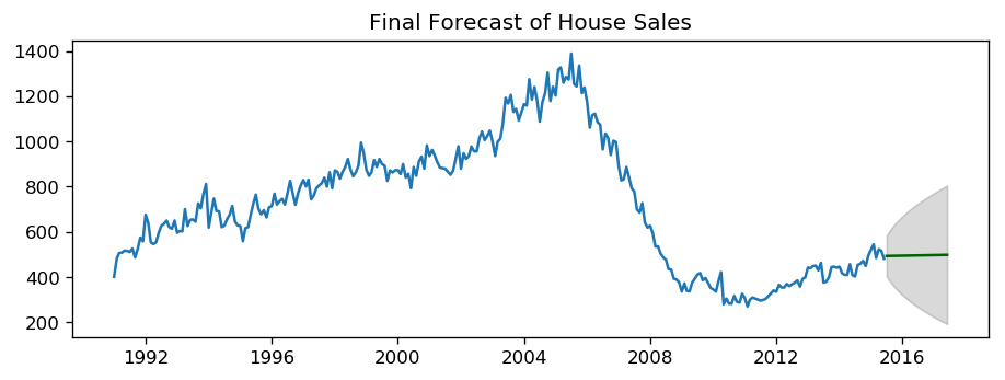
[9]:
ARIMA vs Exponential Smoothing Models
While linear exponential smoothing models are all special cases of ARIMA models, the non-linear exponential smoothing models have no equivalent ARIMA counterparts. On the other hand, there are also many ARIMA models that have no exponential smoothing counterparts. In particular, all exponential smoothing models are non-stationary, while some ARIMA models are stationary.