[1]:
%run ../initscript.py
HTML("""
<div id="popup" style="padding-bottom:5px; display:none;">
    <div>Enter Password:</div>
    <input id="password" type="password"/>
    <button onclick="done()" style="border-radius: 12px;">Submit</button>
</div>
<button onclick="unlock()" style="border-radius: 12px;">Unclock</button>
<a href="#" onclick="code_toggle(this); return false;">show code</a>
""")
[1]:
[2]:
%run ../../notebooks/loadtsfuncs.py
%matplotlib inline
toggle()
[2]:
Forecasting Methods
Forecasting methods can be generally divided into:
Econometric methods
Time series methods
Judgmental Forecasts
Forecasting using judgment is common in practice. In many cases, judgmental forecasting is the only option, such as when there is a complete lack of historical data, or when a new product is being launched, or when a new competitor enters the market, or during completely new and unique market conditions.
Judgmental methods are basically nonquantitative and will not be discussed here. Instead, we will talk about some simple forecasting strategies based on Bayes rule.
Bayes Rule
Bayes Rule can be simply expressed as
\begin{align*} \text{posterior} \propto \text{likelihood} \times \text{prior} \end{align*}
In other words, prediction \(\approx\) observations \(\times\) prior knowledge.
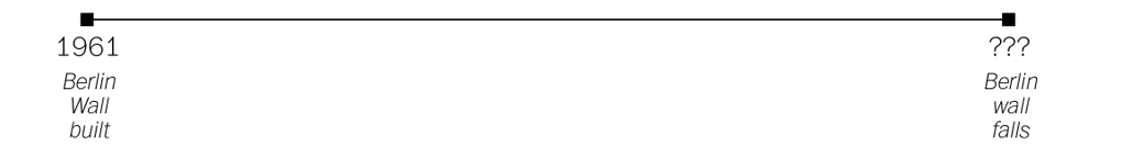
Example: J. Richard Gott III. took a trip to Europe in 1969 and saw the stark symbol of the Cold War — Berlin Wall which had been built eight years earlier in 1961. A question in his mind is “how much longer it would continue to divide the East and West?”.
This may sounds like an absurd prediction. Even setting aside the impossibility of forecasting geopolitics, the question seems mathematically impossible: he needs to make a prediction from a single data point. But as ridiculous as this might seem on its face, we make such predictions all the time by necessity.

John Richard Gott III is a professor of astrophysical sciences at Princeton University.
He is known for developing and advocating two cosmological theories: Time travel and the Doomsday theory.
Gott first thought of his “Copernicus method” of lifetime estimation in 1969 when stopping at the Berlin Wall and wondering how long it would stand.
[3]:
hide_answer()
[3]:
Why it is called the Copernican principle (method)?
In about 1510, the astronomer Nicolaus Copernicus was obsessed by questions: Where are we? Where in the universe is the Earth? Copernicus made a radical imagining at his time that the Earth was not the center of the universe, but, in fact, nowhere special in particular.
When Gott arrived at the Berlin Wall, he asked himself the same question: Where am I? That is to say, where in the total life span of this artifact have I happened to arrive? In a way, he was asking the temporal version of the spatial question that had proposed by Copernicus four hundred years earlier. Gott decided to take the same step with regard to time.
He made the assumption that the moment when he encountered the Berlin Wall was not special. My visit should be located at some random point between the Wall’s beginning and its end.
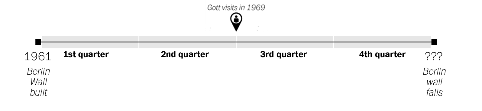
We can divide that timeline up into quarters, like so.
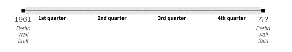
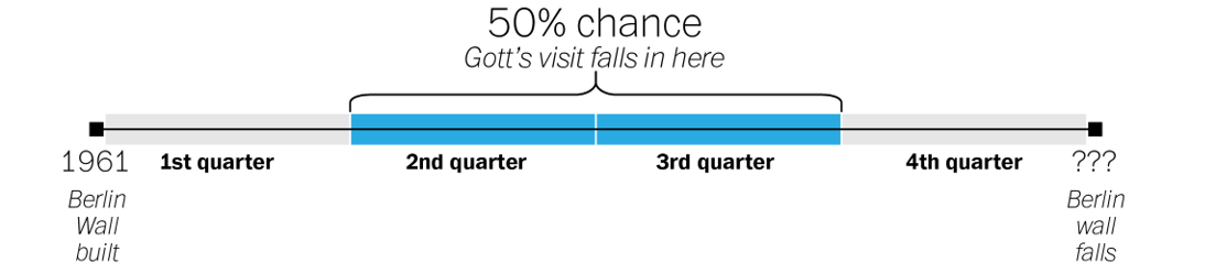
Gott reasoned that his visit, because it was not special in any way, could be located anywhere on that timeline. From the standpoint of probability, that meant there was a 50 percent chance that it was somewhere in the middle portion of the wall’s timeline — the middle two quarters, or 50 percent, of its existence.
When Gott visited in 1969, the Wall had been standing for eight years. If his visit took place at the very beginning of that middle portion of the Wall’s existence, Gott reasoned, that eight years would represent exactly one quarter of the way into its history. That would mean the Wall would exist for another 24 years, coming down in 1993.
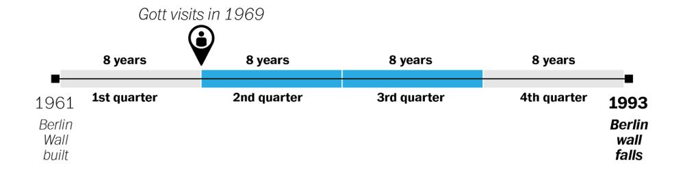
If, on the other hand, his visit happened at the very end of the middle portion, then the eight years would represent exactly three quarters of the way into the Wall’s history. Each quarter would represent just 2.66 years, meaning that the wall could fall as early as 1971.
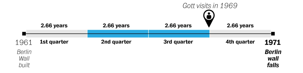
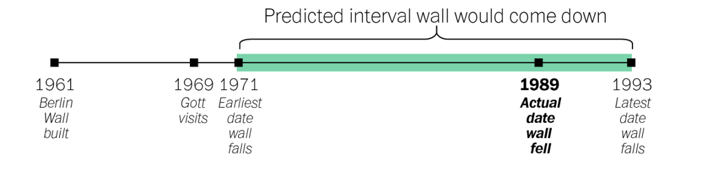
- So by that logic, there was a 50 percent chance that the Wall would come down between 1971 (2.66, or 8/3 years into the future) and 1993 (24, or 8 x 3 years into the future). In reality, the Wall fell in 1989, well within his predicted range.
What if we need a single number prediction instead of a range?
Recall that Gott made the assumption that the moment when he encountered the Berlin Wall wasn’t special–that it was equally likely to be any moment in the wall’s total lifetime. And if any moment was equally likely, then on average his arrival should have come precisely at the halfway point (Why? since it was 50% likely to fall before halfway and 50% likely to fall after).
More generally, unless we know better we can expect to have shown up precisely halfway into the duration of any given phenomenon. And if we assume that we’re arriving precisely halfway into the duration, the best guess we can make for how long it will last into the future becomes obvious: exactly as long as it’s lasted already. Since Gott saw Berlin Wall eight years after it was built, so his best guess was that it would stand for eight years more.
Example: You arrive at a bus stop in a foreign city and learn, perhaps, that the other tourist standing there has been waiting 7 minutes. When is the next bus likely to arrive? Is it worthwhile to wait — and if so, how long should you do so before giving up? 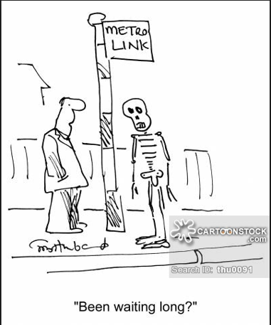
Example: A friend of yours has been dating somebody for ONE Month and wants your advice: is it too soon to invite them along to an upcoming family wedding? The relationship is off to a good start, but how far ahead is it safe to make plans? 
One thing in common for all these examples is that we don’t have much information, or even we have some information, how should we incorporate our information into forecasting. Let’s hold those forecasting questions in mind, and start with some simple math.
Example: There are two different coins. One is a fair coin with a 50–50 chance of heads and tails; the other is a two-headed coin. I drop them into a bag and then pull one out at random. Then I flip it once: head. Which coin do you think I flipped? 
[4]:
hide_answer()
[4]:
There is 100% change to get head for two-headed coin, but only 50% for the normal coin. Thus we can assert confidently that it’s exactly twice as probable, that the friend had pulled out the two headed coin.
Now I show you 9 fair coins and 1 two-headed coin, puts all ten into a bag, draws one at random, and flips it: head. Now what do you suppose? Is it a fair coin or the two-headed one? 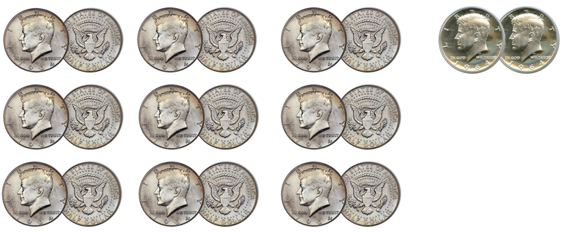
[5]:
hide_answer()
[5]:
As before, a fair coin is exactly half as likely to come up heads as a two-headed coin.
But now, a fair coin is also 9 times as likely to have been drawn in the first place.
Its exactly 4.5 times more likely that your friend is holding a fair coin than the two-headed one.
The number of coins and its probability of showing head are our priors. The outcome of a flip is our observation. We have different predictions when our priors are different.
Is the Copernican Principle Right?
After Gott published his conjecture in Nature, the journal received a flurry of critical correspondence. And it’s easy to see why when we try to apply the rule to some more familiar examples. If you meet a 90-year-old man, the Copernican Principle predicts he will live to 180. Every 6-year-old boy, meanwhile, is predicted to face an early death at the age of 12.
The Copernican Principle is exactly the Bayes Rule by using an uninformative prior. The question is what prior we should use.
Simple Prediction Rules
Average Rule: If our prior information follows normal distribution (things that tend toward or cluster around some kind of natural value), we use the distribution’s “natural” average — its single, specific scale — as your guide.
For example, average life span for men in US is 76 years. So, for a 6-year-old boy, the prediction is 77. He gets a tiny edge over the population average of 76 by virtue of having made it through infancy: we know he is not in the distribution’s left tail.
Multiplicative Rule: If our prior information shows that the rare events have tremendous impact (power-law distribution),
then multiply the quantity observed so far by some constant factor.
For example, movie box-office grosses do not cluster to a “natural” center. Instead, most movies don’t make much money at all, but the occasional Titanic makes titanic amounts. Income (or money in general) is also follows the power-laws (the rich get richer).
For the grosses of movies, the multiplier happens to be 1.4. So if you hear a movie has made $6 million so far, you can guess it will make about $8.4 million overall.
This multiplicative rule is a direct consequence of the fact that power-law distributions do not specify (or you are uninformative on) a natural scale for the phenomenon they are describing. It is possible that a movie that is grossed $6 million is actually a blockbuster in its first hour of release, but it is far more likely to be just a single-digit-millions kind of movie.
In summary, something normally distributed that’s gone on seemingly too long is bound to end shortly; but the longer something in a power-law distribution has gone on, the longer you can expect it to keep going.
There’s a third category of things in life: those that are neither more nor less likely to end just because they have gone on for a while.
Additive Rule: If the prior follows Erlang distributions (e.g. exponential or gamma distributions), then we should always predict that things will go on just a constant amount longer. It is a memoryless prediction.
Additive rule is suitable for events that are completely independent from one another and the intervals between them thus fall on Erlang distribution.
If you wait for a win at the roulette wheel, what is your strategy?
[6]:
hide_answer()
[6]:
Suppose a win at the roulette wheel were characterized by a normal distribution, then the Average Rule would apply: after a run of bad luck, it’d tell you that your number should be coming any second, probably followed by more losing spins. The strategy is to quit after winning.
If, instead, the wait for a win obeyed a power-law distribution, then the Multiplicative Rule would tell you that winning spins follow quickly after one another, but the longer a drought had gone on the longer it would probably continue. The strategy is keep playing for a while after any win, but give up after a losing streak.
If it is a memoryless distribution, then you’re stuck. The Additive Rule tells you the chance of a win now is the same as it was an hour ago, and the same as it will be an hour from now. Nothing ever changes. You’re not rewarded for sticking it out and ending on a high note; neither is there a tipping point when you should just cut your losses. For a memoryless distribution, there is no right time to quit. This may in part explain these games’ addictiveness.
In summary, knowing what distribution you’re up against (i.e. having a correct prior knowledge) can make all the difference.
Small Data is Big Data in Disguise
Many behavior studies show that the predictions that people had made were extremely close to those produced by Bayes Rule.
The reason we can often make good predictions from a small number of observations — or just a single one — is that our priors are so rich.
Behavior studies show that we actually carry around in our heads surprisingly accurate priors.
However, the challenge has increased with the development of the printing press, the nightly news, and social media. Those innovations allow us to spread information mechanically which may affect our priors.
As sociologist Barry Glassner notes, the murder rate in the United States declined by 20% over the course of the 1990s, yet during that time period the presence of gun violence on American news increased by 600%.
If you want to naturally make good predictions by following your intuitions, without having to think about what kind of prediction rule is appropriate, you need to protect your priors. Counter-intuitively, that might mean turning off the news.
Fitting and Forecasting
We have 12 data points that are generated from \(\sin(2 \pi x)\) with some small perturbations.
[7]:
interact(training_data,
         show=widgets.Checkbox(value=False, description='Original', disabled=False));
Our task is to foresee (forecast) the underlying data pattern, which is \(\sin(2 \pi x)\), based on given 12 observations. Note
The function \(\sin(2 \pi x)\) is the information we are trying to obtain
The perturbations are noises that we do not want to extract
Remember that we only observe training data without knowing anything about underlying generating function \(\sin(2 \pi x)\) and perturbations. Suppose we try to interpret the data by polynomial functions with degree 1 (linear regression), 3 and 9.
[8]:
interact(poly_fit,
         show=widgets.Checkbox(value=False, description='Original', disabled=False));
With knowing the underlying true function \(\sin(2 \pi x)\), it is clear that
the linear regression is under-fitting because it doesn’t explain the up-and-down pattern in the data;
the polynomial function with degree 9 is over-fitting because it focuses too much on noises and does not correctly interpret the pattern in the data;
the polynomial with degree 3 is the best because it balances the information and noises and extracts the valuable information from the data.
However, is it possible to identify that a polynomial with degree 3 is the best without knowing the underlying true function?
Yes. We can use holdout as follows:
choose 3 data points as testing data
fit polynomial functions only on the remaining 9 data points
find the best fitting function based on the testing data
[9]:
interact(poly_fit_holdout,
         show=widgets.Checkbox(value=False, description='Original', disabled=False),
         train=widgets.Checkbox(value=True, description='Training Data', disabled=False),
         test=widgets.Checkbox(value=False, description='Testing Data', disabled=False));
Occam’s razor the law of parsimony: we generally prefer a simpler model because simpler models track only the most basic underlying patterns and can be more flexible and accurate in forecasting the future!