[1]:
%run ../initscript.py
HTML("""
<div id="popup" style="padding-bottom:5px; display:none;">
<div>Enter Password:</div>
<input id="password" type="password"/>
<button onclick="done()" style="border-radius: 12px;">Submit</button>
</div>
<button onclick="unlock()" style="border-radius: 12px;">Unclock</button>
<a href="#" onclick="code_toggle(this); return false;">show code</a>
""")
[1]:
[2]:
%run ../../notebooks/loadtsfuncs.py
%matplotlib inline
toggle()
[2]:
Components of Time Series
Depending on the nature of the trend and seasonality, we have
Additive Model:
\[\text{Data = Seasonal effect + Trend-Cyclical + Residual}\]Multiplicative Model:
\[\text{Data = Seasonal effect $\times$ Trend-Cyclical $\times$ Residual}\]
Note a multiplicative model is additive after a logrithmic transform because
Besides trend, seasonality and error, another aspect to consider is the cyclic behaviour. It happens when the rise and fall pattern in the series does not happen in fixed calendar-based intervals. Care should be taken to not confuse ‘cyclic’ effect with ‘seasonal’ effect.
Cyclic vs Seasonal Pattern
A seasonal pattern exists when a series is influenced by seasonal factors (e.g., the quarter of the year, the month, or day of the week). Seasonality is always of a fixed and known period.
A seasonal behavior is very strictly regular, meaning there is a precise amount of time between the peaks and troughs of the data. For instance temperature would have a seasonal behavior. The coldest day of the year and the warmest day of the year may move (because of factors other than time than influence the data) but you will never see drift over time where eventually winter comes in June in the northern hemisphere.
A cyclic pattern exists when data exhibit rises and falls that are not of fixed period.
Cyclical behavior on the other hand can drift over time because the time between periods isn’t precise. For example, the stock market tends to cycle between periods of high and low values, but there is no set amount of time between those fluctuations.
Some examples about cyclic vs seasonal pattern:
[3]:
hide_answer()
[3]:
Series can show both cyclical and seasonal behavior.
Considering the home prices, there is a cyclical effect due to the market, but there is also a seasonal effect because most people would rather move in the summer when their kids are between grades of school.
You can also have multiple seasonal (or cyclical) effects.
For example, people tend to try and make positive behavioral changes on the “1st” of something, so you see spikes in gym attendance of course on the 1st of the year, but also the first of each month and each week, so gym attendance has yearly, monthly, and weekly seasonality.
When you are looking for a second seasonal pattern or a cyclical pattern in seasonal data, it can help to take a moving average at the higher seasonal frequency to remove those seasonal effects. For instance, if you take a moving average of the housing data with a window size of 12 you will see the cyclical pattern more clearly. This only works though to remove a higher frequency pattern from a lower frequency one.
Seasonal behavior does not have to happen only on sub-year time units.
For example, the sun goes through what are called “solar cycles” which are periods of time where it puts out more or less heat. This behavior shows a seasonality of almost exactly 11 years, so a yearly time series of the heat put out by the sun would have a seasonality of 11.
In many cases the difference in seasonal vs cyclical behavior can be known or measured with reasonable accuracy by looking at the regularity of the peaks in your data and looking for a drift the timing peaks from the mean distance between them.
A series with strong seasonality will show clear peaks in the partial auto-correlation function as well as the auto-correlation function, whereas a cyclical series will only have the strong peaks in the auto-correlation function.
However if you don’t have enough data to determine this or if the data is very noisy making the measurements difficult, the best way to determine if a behavior is cyclical or seasonal can be thinking about the cause of the fluctuation in the data.
If the cause is dependent directly on time then the data are likely seasonal (ex. it takes ~365.25 days for the earth to travel around the sun, the position of the earth around the sun effects temperature, therefore temperature shows a yearly seasonal pattern).
If on the other hand, the cause is based on previous values of the series rather than directly on time, the series is likely cyclical (ex. when the value of stocks go up, it gives confidence in the market, so more people invest making prices go up, and vice versa, therefore stocks show a cyclical pattern).
The class of exponential smoothing allows for seasonality but not cyclicity. The class of ARMA models can handle both seasonality and cyclic behavior, but long-period cyclicity is not handled very well in the ARMA framework.
Decompose a Time Series
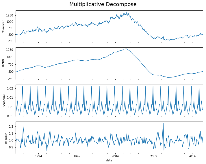
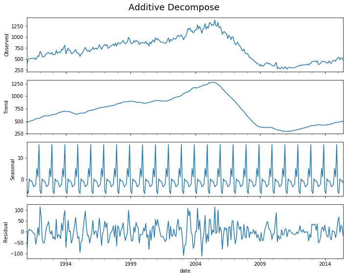
[4]:
decomp(df_house.sales)
Multiplicative Model : Observed 401.000 = (Seasonal 479.897 * Trend 0.996 * Resid 0.839)
Additive Model : Observed 401.000 = (Seasonal 479.897 + Trend -5.321 + Resid -73.576)
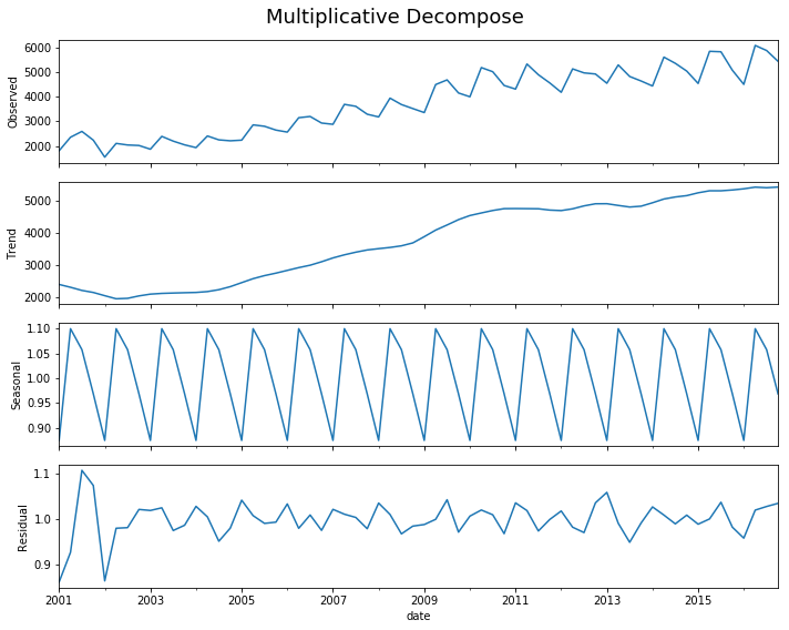
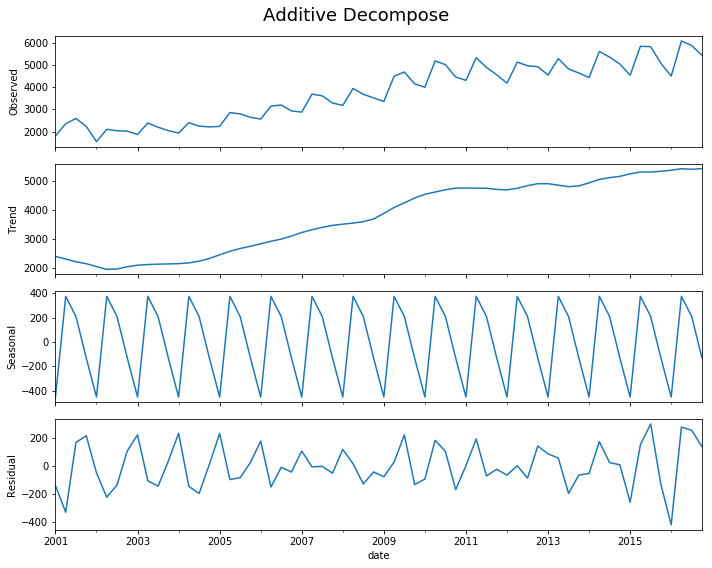
[5]:
decomp(df_drink.sales)
Multiplicative Model : Observed 1807.370 = (Seasonal 2401.083 * Trend 0.875 * Resid 0.861)
Additive Model : Observed 1807.370 = (Seasonal 2401.083 + Trend -452.058 + Resid -141.655)
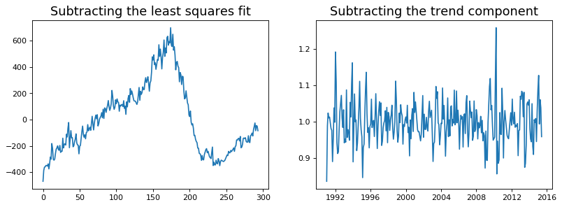
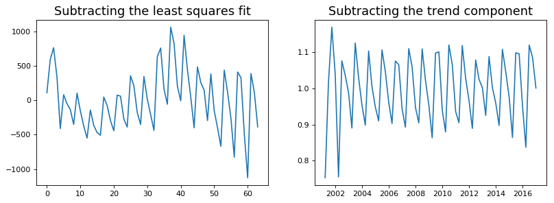
Detrend a Time Series
There are multiple approaches to remove the trend component from a time series:
Subtract the line of best fit from the time series. The line of best fit may be obtained from a linear regression model with the time steps as the predictor. For more complex trends, we can also add quadratic terms \(x^2\) in the model.
Subtract the trend component obtained from time series decomposition we saw earlier.
Subtract the mean
We implement the first two methods. It is clear that the line of best fit is not enough to detrend the data.
[6]:
detrend(df_house['sales'])
[7]:
detrend(df_drink['sales'])
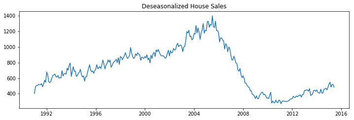
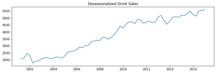
Deseasonalize a Time Series
There are multiple approaches to deseasonalize a time series: 1. Take a moving average with length as the seasonal window. This will smoothen in series in the process. 2. Seasonal difference the series (subtract the value of previous season from the current value) 3. Divide the series by the seasonal index obtained from STL decomposition
If dividing by the seasonal index does not work well, try taking a log of the series and then do the deseasonalizing. You can later restore to the original scale by taking an exponential.
[8]:
deseasonalize(df_house.sales, model='multiplicative', title='House Sales')
[9]:
deseasonalize(df_drink.sales, model='multiplicative', title='Drink Sales')
Test for Seasonality
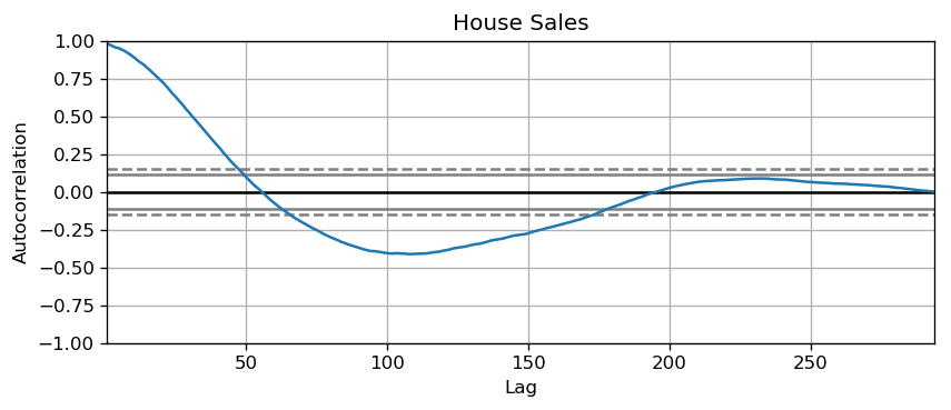
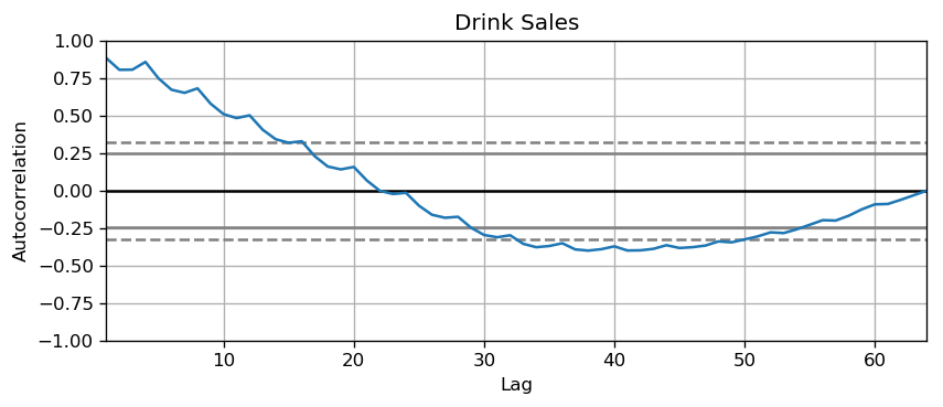
The common way is to plot the series and check for repeatable patterns in fixed time intervals. However, if you want a more definitive inspection of the seasonality, use the Autocorrelation Function (ACF) plot. Strong patterns in real word datasets is hardly noticed and can get distorted by any noise, so you need a careful eye to capture these patterns.
Alternately, if you want a statistical test, the Canova-Hansen test for seasonal differences can determine if seasonal differencing is required to stationarize the series.
[10]:
plot_autocorr(df_house.sales,'House Sales')
[11]:
plot_autocorr(df_drink.sales,'Drink Sales')
Missing Values in a Time Series
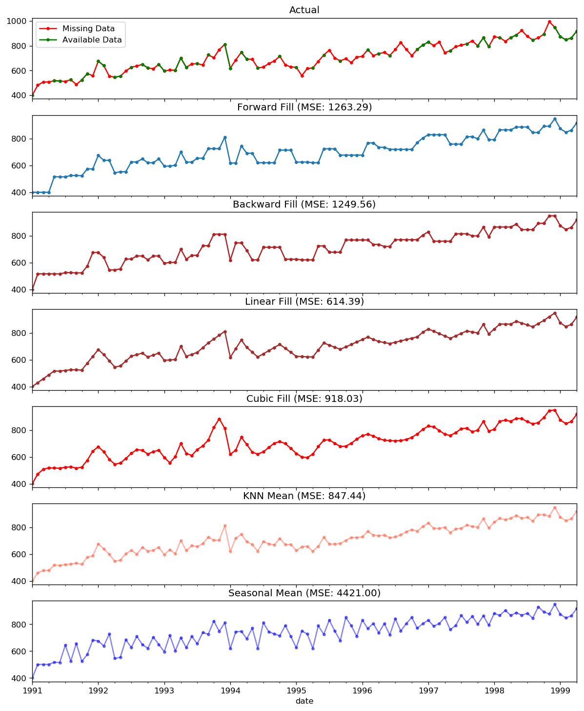
When the time series have missing dates or times, the data was not captured or available for those periods. We may need to fill up those periods with a reasonable value. It is typically not a good idea to replace missing values with the mean of the series, especially if the series is not stationary.
Depending on the nature of the series, there are a few approaches are available:
Forward Fill
Backward Fill
Linear Interpolation
Quadratic interpolation
Mean of nearest neighbors
Mean of seasonal couterparts
In the demonstration, we manually introduce missing values to the time series and impute it with above approaches. Since the original non-missing values are known, we can measure the imputation performance by calculating the mean squared error (MSE) of the imputed against the actual values.
More interesting approaches can be considered:
If explanatory variables are available, we can use a prediction model such as the random forest or k-Nearest Neighbors to predict missing values.
If past observations are enough, we can forecast the missing values.
If future observations are enough, we can backcast the missing values
We can also forecast the counterparts from previous cycles.
[12]:
from scipy.interpolate import interp1d
from sklearn.metrics import mean_squared_error
dataurl = 'https://raw.githubusercontent.com/ming-zhao/Business-Analytics/master/data/time_series/'
# for easy demonstration, we only consider 100 observations
df_orig = pd.read_csv(dataurl+'house_sales.csv', parse_dates=['date'], index_col='date').head(100)
df_missing = pd.read_csv(dataurl+'house_sales_missing.csv', parse_dates=['date'], index_col='date')
fig, axes = plt.subplots(7, 1, sharex=True, figsize=(12, 15))
plt.rcParams.update({'xtick.bottom' : False})
## 1. Actual -------------------------------
df_orig.plot(y="sales", title='Actual', ax=axes[0], label='Actual', color='red', style=".-")
df_missing.plot(y="sales", title='Actual', ax=axes[0], label='Actual', color='green', style=".-")
axes[0].legend(["Missing Data", "Available Data"])
## 2. Forward Fill --------------------------
df_ffill = df_missing.ffill()
error = np.round(mean_squared_error(df_orig['sales'], df_ffill['sales']), 2)
df_ffill['sales'].plot(title='Forward Fill (MSE: ' + str(error) +")",
ax=axes[1], label='Forward Fill', style=".-")
## 3. Backward Fill -------------------------
df_bfill = df_missing.bfill()
error = np.round(mean_squared_error(df_orig['sales'], df_bfill['sales']), 2)
df_bfill['sales'].plot(title="Backward Fill (MSE: " + str(error) +")",
ax=axes[2], label='Back Fill', color='firebrick', style=".-")
## 4. Linear Interpolation ------------------
df_missing['rownum'] = np.arange(df_missing.shape[0])
df_nona = df_missing.dropna(subset = ['sales'])
f = interp1d(df_nona['rownum'], df_nona['sales'])
df_missing['linear_fill'] = f(df_missing['rownum'])
error = np.round(mean_squared_error(df_orig['sales'], df_missing['linear_fill']), 2)
df_missing['linear_fill'].plot(title="Linear Fill (MSE: " + str(error) +")",
ax=axes[3], label='Cubic Fill', color='brown', style=".-")
## 5. Cubic Interpolation --------------------
f2 = interp1d(df_nona['rownum'], df_nona['sales'], kind='cubic')
df_missing['cubic_fill'] = f2(df_missing['rownum'])
error = np.round(mean_squared_error(df_orig['sales'], df_missing['cubic_fill']), 2)
df_missing['cubic_fill'].plot(title="Cubic Fill (MSE: " + str(error) +")",
ax=axes[4], label='Cubic Fill', color='red', style=".-")
# Interpolation References:
# https://docs.scipy.org/doc/scipy/reference/tutorial/interpolate.html
# https://docs.scipy.org/doc/scipy/reference/interpolate.html
## 6. Mean of 'n' Nearest Past Neighbors ------
def knn_mean(ts, n):
out = np.copy(ts)
for i, val in enumerate(ts):
if np.isnan(val):
n_by_2 = np.ceil(n/2)
lower = np.max([0, int(i-n_by_2)])
upper = np.min([len(ts)+1, int(i+n_by_2)])
ts_near = np.concatenate([ts[lower:i], ts[i:upper]])
out[i] = np.nanmean(ts_near)
return out
df_missing['knn_mean'] = knn_mean(df_missing['sales'].values, 8)
error = np.round(mean_squared_error(df_orig['sales'], df_missing['knn_mean']), 2)
df_missing['knn_mean'].plot(title="KNN Mean (MSE: " + str(error) +")",
ax=axes[5], label='KNN Mean', color='tomato', alpha=0.5, style=".-")
# 7. Seasonal Mean ----------------------------
def seasonal_mean(ts, n, lr=0.7):
"""
Compute the mean of corresponding seasonal periods
ts: 1D array-like of the time series
n: Seasonal window length of the time series
"""
out = np.copy(ts)
for i, val in enumerate(ts):
if np.isnan(val):
ts_seas = ts[i-1::-n] # previous seasons only
out[i] = out[i-1]
if ~ts_seas.isnull().all():
if np.isnan(np.nanmean(ts_seas)):
ts_seas = np.concatenate([ts[i-1::-n], ts[i::n]]) # previous and forward
out[i] = np.nanmean(ts_seas) * lr
return out
df_missing['seasonal_mean'] = seasonal_mean(df_missing['sales'], n=6, lr=1.25)
error = np.round(mean_squared_error(df_orig['sales'], df_missing['seasonal_mean']), 2)
df_missing['seasonal_mean'].plot(title="Seasonal Mean (MSE: {:.2f})".format(error),
ax=axes[6], label='Seasonal Mean', color='blue', alpha=0.5, style=".-")
plt.show()
toggle()
[12]: