[1]:
%run ../initscript.py
HTML("""
<div id="popup" style="padding-bottom:5px; display:none;">
<div>Enter Password:</div>
<input id="password" type="password"/>
<button onclick="done()" style="border-radius: 12px;">Submit</button>
</div>
<button onclick="unlock()" style="border-radius: 12px;">Unclock</button>
<a href="#" onclick="code_toggle(this); return false;">show code</a>
""")
[1]:
[2]:
%run ../../notebooks/loadtsfuncs.py
%matplotlib inline
toggle()
[2]:
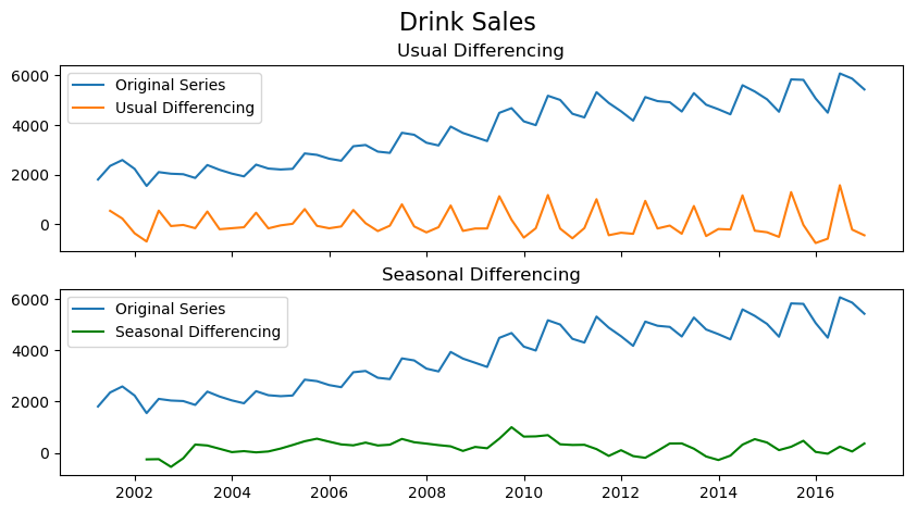
Seasonal ARIMA (SARIMA) Models
The ARIMA model does not support seasonality. If the time series data has defined seasonality, then we need to perform seasonal differencing and SARIMA models.
Seasonal differencing is similar to regular differencing, but, instead of subtracting consecutive terms, we subtract the value from previous season.
The model is represented as SARIMA\((p,d,q)x(P,D,Q)\), where - \(D\) is the order of seasonal differencing - \(P\) is the order of seasonal autoregression (SAR) - \(Q\) is the order of seasonal moving average (SMA) - \(x\) is the frequency of the time series.
[3]:
fig, axes = plt.subplots(2, 1, figsize=(10,5), dpi=100, sharex=True)
# Usual Differencing
axes[0].plot(df_drink.sales, label='Original Series')
axes[0].plot(df_drink.sales.diff(1), label='Usual Differencing')
axes[0].set_title('Usual Differencing')
axes[0].legend(loc='upper left', fontsize=10)
# Seasinal Differencing
axes[1].plot(df_drink.sales, label='Original Series')
axes[1].plot(df_drink.sales.diff(4), label='Seasonal Differencing', color='green')
axes[1].set_title('Seasonal Differencing')
plt.legend(loc='upper left', fontsize=10)
plt.suptitle('Drink Sales', fontsize=16)
plt.show()
toggle()
[3]:
As we can clearly see, the seasonal spikes is intact after applying usual differencing (lag 1). Whereas, it is rectified after seasonal differencing.
Build SARIMA Model
Find optimal SARIMA for house sales:
[4]:
sarima_house = pm.auto_arima(df_house.sales,
start_p=1, start_q=1,
test='adf',
max_p=3, max_q=3, m=4,
start_P=0, seasonal=True,
d=None, D=1, trace=True,
error_action='ignore',
suppress_warnings=True,
stepwise=True)
sarima_house.summary()
Fit ARIMA: order=(1, 0, 1) seasonal_order=(0, 1, 1, 4); AIC=3069.410, BIC=3087.760, Fit time=0.762 seconds
Fit ARIMA: order=(0, 0, 0) seasonal_order=(0, 1, 0, 4); AIC=3317.294, BIC=3324.633, Fit time=0.031 seconds
Fit ARIMA: order=(1, 0, 0) seasonal_order=(1, 1, 0, 4); AIC=3167.461, BIC=3182.140, Fit time=1.203 seconds
Fit ARIMA: order=(0, 0, 1) seasonal_order=(0, 1, 1, 4); AIC=3242.302, BIC=3256.981, Fit time=0.726 seconds
Fit ARIMA: order=(1, 0, 1) seasonal_order=(1, 1, 1, 4); AIC=3068.582, BIC=3090.601, Fit time=1.706 seconds
Fit ARIMA: order=(1, 0, 1) seasonal_order=(1, 1, 0, 4); AIC=3144.942, BIC=3163.292, Fit time=1.418 seconds
Fit ARIMA: order=(1, 0, 1) seasonal_order=(1, 1, 2, 4); AIC=3068.586, BIC=3094.275, Fit time=2.691 seconds
Fit ARIMA: order=(1, 0, 1) seasonal_order=(0, 1, 0, 4); AIC=3236.794, BIC=3251.474, Fit time=0.259 seconds
Fit ARIMA: order=(1, 0, 1) seasonal_order=(2, 1, 2, 4); AIC=3071.836, BIC=3101.195, Fit time=3.053 seconds
Fit ARIMA: order=(0, 0, 1) seasonal_order=(1, 1, 1, 4); AIC=3235.957, BIC=3254.306, Fit time=0.686 seconds
Fit ARIMA: order=(2, 0, 1) seasonal_order=(1, 1, 1, 4); AIC=3070.496, BIC=3096.185, Fit time=0.732 seconds
Fit ARIMA: order=(1, 0, 0) seasonal_order=(1, 1, 1, 4); AIC=3090.901, BIC=3109.250, Fit time=0.514 seconds
Fit ARIMA: order=(1, 0, 2) seasonal_order=(1, 1, 1, 4); AIC=3070.548, BIC=3096.237, Fit time=1.153 seconds
Fit ARIMA: order=(0, 0, 0) seasonal_order=(1, 1, 1, 4); AIC=3313.310, BIC=3327.989, Fit time=0.344 seconds
Fit ARIMA: order=(2, 0, 2) seasonal_order=(1, 1, 1, 4); AIC=nan, BIC=nan, Fit time=nan seconds
Fit ARIMA: order=(1, 0, 1) seasonal_order=(2, 1, 1, 4); AIC=3069.171, BIC=3094.860, Fit time=0.923 seconds
Total fit time: 16.243 seconds
[4]:
| Dep. Variable: | y | No. Observations: | 294 |
|---|---|---|---|
| Model: | SARIMAX(1, 0, 1)x(1, 1, 1, 4) | Log Likelihood | -1528.291 |
| Date: | Wed, 15 May 2019 | AIC | 3068.582 |
| Time: | 11:51:11 | BIC | 3090.601 |
| Sample: | 0 | HQIC | 3077.404 |
| - 294 | |||
| Covariance Type: | opg |
| coef | std err | z | P>|z| | [0.025 | 0.975] | |
|---|---|---|---|---|---|---|
| intercept | 0.0002 | 0.129 | 0.002 | 0.998 | -0.254 | 0.254 |
| ar.L1 | 0.9997 | 0.143 | 6.994 | 0.000 | 0.720 | 1.280 |
| ma.L1 | -0.3049 | 0.053 | -5.765 | 0.000 | -0.409 | -0.201 |
| ar.S.L4 | -0.1031 | 0.056 | -1.848 | 0.065 | -0.212 | 0.006 |
| ma.S.L4 | -0.9982 | 0.647 | -1.542 | 0.123 | -2.267 | 0.271 |
| sigma2 | 2109.4165 | 1043.105 | 2.022 | 0.043 | 64.968 | 4153.865 |
| Ljung-Box (Q): | 68.41 | Jarque-Bera (JB): | 5.09 |
|---|---|---|---|
| Prob(Q): | 0.00 | Prob(JB): | 0.08 |
| Heteroskedasticity (H): | 0.55 | Skew: | -0.14 |
| Prob(H) (two-sided): | 0.00 | Kurtosis: | 3.59 |
Warnings:
[1] Covariance matrix calculated using the outer product of gradients (complex-step).
Find optimal SARIMA for drink sales
[5]:
sarima_drink = pm.auto_arima(df_drink.sales,
start_p=1, start_q=1,
test='adf',
max_p=3, max_q=3, m=4,
start_P=0, seasonal=True,
d=None, D=1, trace=True,
error_action='ignore',
suppress_warnings=True,
stepwise=True)
sarima_drink.summary()
Fit ARIMA: order=(1, 0, 1) seasonal_order=(0, 1, 1, 4); AIC=809.758, BIC=820.230, Fit time=0.281 seconds
Fit ARIMA: order=(0, 0, 0) seasonal_order=(0, 1, 0, 4); AIC=848.072, BIC=852.261, Fit time=0.021 seconds
Fit ARIMA: order=(1, 0, 0) seasonal_order=(1, 1, 0, 4); AIC=813.490, BIC=821.867, Fit time=0.088 seconds
Fit ARIMA: order=(0, 0, 1) seasonal_order=(0, 1, 1, 4); AIC=813.808, BIC=822.185, Fit time=0.233 seconds
Fit ARIMA: order=(1, 0, 1) seasonal_order=(1, 1, 1, 4); AIC=811.146, BIC=823.712, Fit time=0.483 seconds
Fit ARIMA: order=(1, 0, 1) seasonal_order=(0, 1, 0, 4); AIC=810.383, BIC=818.760, Fit time=0.152 seconds
Fit ARIMA: order=(1, 0, 1) seasonal_order=(0, 1, 2, 4); AIC=811.498, BIC=824.064, Fit time=0.230 seconds
Fit ARIMA: order=(1, 0, 1) seasonal_order=(1, 1, 2, 4); AIC=813.467, BIC=828.127, Fit time=0.337 seconds
Fit ARIMA: order=(2, 0, 1) seasonal_order=(0, 1, 1, 4); AIC=811.201, BIC=823.767, Fit time=0.322 seconds
Fit ARIMA: order=(1, 0, 0) seasonal_order=(0, 1, 1, 4); AIC=813.022, BIC=821.399, Fit time=0.152 seconds
Fit ARIMA: order=(1, 0, 2) seasonal_order=(0, 1, 1, 4); AIC=810.926, BIC=823.492, Fit time=0.402 seconds
Fit ARIMA: order=(0, 0, 0) seasonal_order=(0, 1, 1, 4); AIC=849.704, BIC=855.987, Fit time=0.084 seconds
Fit ARIMA: order=(2, 0, 2) seasonal_order=(0, 1, 1, 4); AIC=813.065, BIC=827.725, Fit time=0.872 seconds
Total fit time: 3.670 seconds
[5]:
| Dep. Variable: | y | No. Observations: | 64 |
|---|---|---|---|
| Model: | SARIMAX(1, 0, 1)x(0, 1, 1, 4) | Log Likelihood | -399.879 |
| Date: | Wed, 15 May 2019 | AIC | 809.758 |
| Time: | 11:51:14 | BIC | 820.230 |
| Sample: | 0 | HQIC | 813.854 |
| - 64 | |||
| Covariance Type: | opg |
| coef | std err | z | P>|z| | [0.025 | 0.975] | |
|---|---|---|---|---|---|---|
| intercept | 121.9284 | 50.994 | 2.391 | 0.017 | 21.981 | 221.876 |
| ar.L1 | 0.4436 | 0.178 | 2.492 | 0.013 | 0.095 | 0.793 |
| ma.L1 | 0.5287 | 0.143 | 3.687 | 0.000 | 0.248 | 0.810 |
| ma.S.L4 | -0.2772 | 0.141 | -1.969 | 0.049 | -0.553 | -0.001 |
| sigma2 | 3.487e+04 | 6857.056 | 5.085 | 0.000 | 2.14e+04 | 4.83e+04 |
| Ljung-Box (Q): | 28.74 | Jarque-Bera (JB): | 0.83 |
|---|---|---|---|
| Prob(Q): | 0.91 | Prob(JB): | 0.66 |
| Heteroskedasticity (H): | 1.28 | Skew: | -0.29 |
| Prob(H) (two-sided): | 0.58 | Kurtosis: | 3.03 |
Warnings:
[1] Covariance matrix calculated using the outer product of gradients (complex-step).
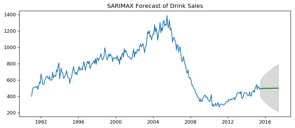
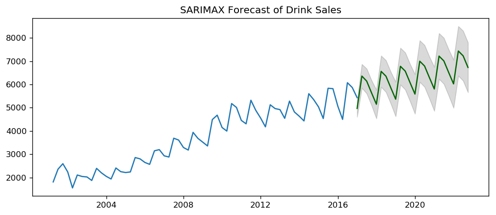
SARIMA Forecast
[6]:
sarima_forcast(sarima_house, df_house, 'sales', forecast_periods=24, freq='month')
[7]:
sarima_forcast(sarima_drink, df_drink, 'sales', forecast_periods=24, freq='quarter')
SARIMAX Model with Exogenous Variable
We have a SARIMA model if there is an external predictor, also called, “exogenous variable” built into SARIMA models. The only requirement to use an exogenous variable is that we need to know the value of the variable during the forecast period as well.
For the sake of demonstration, we use the seasonal index from the classical seasonal decomposition on the latest 3 years of data even though SARIMA already modeling the seasonality.
The seasonal index is a good exogenous variable for demonstration purpose because it repeats every frequency cycle, 4 quarters in this case. So, we always know what values the seasonal index will hold for the future forecasts.
[8]:
df_drink = add_seasonal_index(df_drink, 'sales', freq='quarter', model='multiplicative')
sarimax_drink = pm.auto_arima(df_drink[['sales']], exogenous=df_drink[['seasonal_index']],
start_p=1, start_q=1,
test='adf',
max_p=3, max_q=3, m=12,
start_P=0, seasonal=True,
d=None, D=1, trace=True,
error_action='ignore',
suppress_warnings=True,
stepwise=True)
sarimax_drink.summary()
Fit ARIMA: order=(1, 1, 1) seasonal_order=(0, 1, 1, 12); AIC=727.512, BIC=739.103, Fit time=0.557 seconds
Fit ARIMA: order=(0, 1, 0) seasonal_order=(0, 1, 0, 12); AIC=730.208, BIC=736.003, Fit time=0.025 seconds
Fit ARIMA: order=(1, 1, 0) seasonal_order=(1, 1, 0, 12); AIC=726.746, BIC=736.405, Fit time=0.512 seconds
Fit ARIMA: order=(0, 1, 1) seasonal_order=(0, 1, 1, 12); AIC=728.526, BIC=738.185, Fit time=0.368 seconds
Fit ARIMA: order=(1, 1, 0) seasonal_order=(0, 1, 0, 12); AIC=732.167, BIC=739.895, Fit time=0.039 seconds
Fit ARIMA: order=(1, 1, 0) seasonal_order=(2, 1, 0, 12); AIC=728.728, BIC=740.319, Fit time=1.604 seconds
Fit ARIMA: order=(1, 1, 0) seasonal_order=(1, 1, 1, 12); AIC=nan, BIC=nan, Fit time=nan seconds
Fit ARIMA: order=(1, 1, 0) seasonal_order=(2, 1, 1, 12); AIC=nan, BIC=nan, Fit time=nan seconds
Fit ARIMA: order=(0, 1, 0) seasonal_order=(1, 1, 0, 12); AIC=724.752, BIC=732.479, Fit time=0.346 seconds
Fit ARIMA: order=(0, 1, 1) seasonal_order=(1, 1, 0, 12); AIC=726.648, BIC=736.307, Fit time=0.451 seconds
Fit ARIMA: order=(1, 1, 1) seasonal_order=(1, 1, 0, 12); AIC=728.330, BIC=739.921, Fit time=0.477 seconds
Fit ARIMA: order=(0, 1, 0) seasonal_order=(2, 1, 0, 12); AIC=726.757, BIC=736.416, Fit time=0.502 seconds
Fit ARIMA: order=(0, 1, 0) seasonal_order=(1, 1, 1, 12); AIC=nan, BIC=nan, Fit time=nan seconds
Fit ARIMA: order=(0, 1, 0) seasonal_order=(2, 1, 1, 12); AIC=nan, BIC=nan, Fit time=nan seconds
Total fit time: 4.916 seconds
[8]:
| Dep. Variable: | y | No. Observations: | 64 |
|---|---|---|---|
| Model: | SARIMAX(0, 1, 0)x(1, 1, 0, 12) | Log Likelihood | -358.376 |
| Date: | Wed, 15 May 2019 | AIC | 724.752 |
| Time: | 11:51:20 | BIC | 732.479 |
| Sample: | 0 | HQIC | 727.705 |
| - 64 | |||
| Covariance Type: | opg |
| coef | std err | z | P>|z| | [0.025 | 0.975] | |
|---|---|---|---|---|---|---|
| intercept | 5.4344 | 44.502 | 0.122 | 0.903 | -81.787 | 92.656 |
| x1 | -0.0406 | 3.01e+04 | -1.35e-06 | 1.000 | -5.9e+04 | 5.9e+04 |
| ar.S.L12 | -0.4401 | 0.151 | -2.922 | 0.003 | -0.735 | -0.145 |
| sigma2 | 7.164e+04 | 1.95e+04 | 3.671 | 0.000 | 3.34e+04 | 1.1e+05 |
| Ljung-Box (Q): | 52.27 | Jarque-Bera (JB): | 2.60 |
|---|---|---|---|
| Prob(Q): | 0.09 | Prob(JB): | 0.27 |
| Heteroskedasticity (H): | 1.70 | Skew: | 0.54 |
| Prob(H) (two-sided): | 0.28 | Kurtosis: | 2.74 |
Warnings:
[1] Covariance matrix calculated using the outer product of gradients (complex-step).
[9]:
sarimax_forcast(sarimax_drink, df_drink, 'sales', forecast_periods=24, freq='quarter')
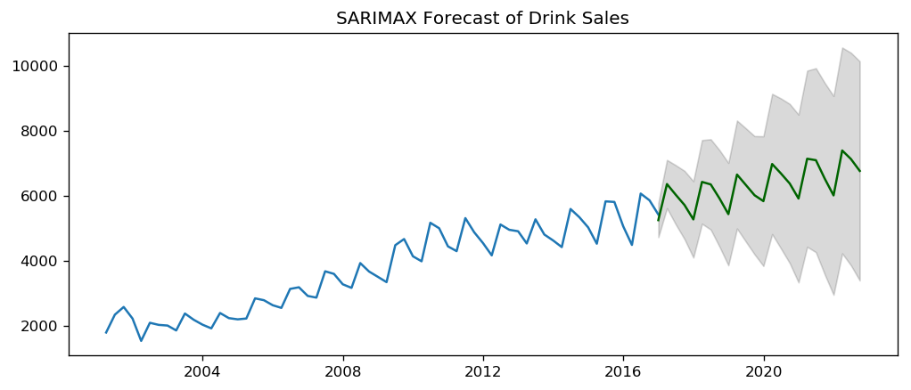
The coefficient of x1 is small and p-value is large, so the contribution from seasonal index is negligible.