%run ../initscript.py
HTML("""
<div id="popup" style="padding-bottom:5px; display:none;">
    <div>Enter Password:</div>
    <input id="password" type="password"/>
    <button onclick="done()" style="border-radius: 12px;">Submit</button>
</div>
<button onclick="unlock()" style="border-radius: 12px;">Unclock</button>
<a href="#" onclick="code_toggle(this); return false;">show code</a>
""")

Enter Password:

Submit

Unclock show code

%run ../../notebooks/loadtsfuncs.py
%matplotlib inline
toggle()

show code

Autocorrelation and Partial Autocorrelation Functions

Autocorrelation

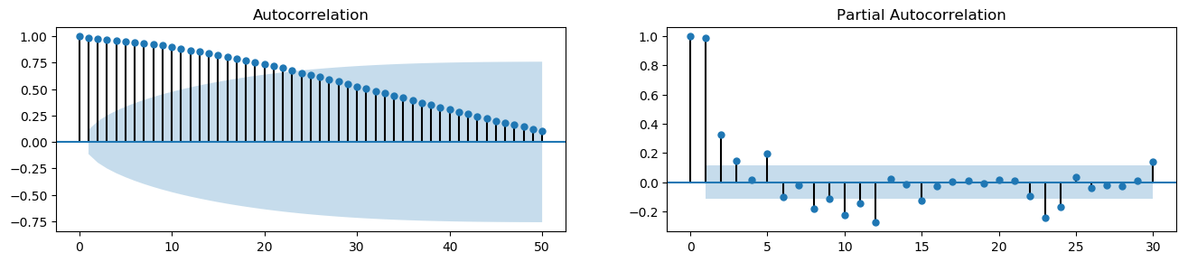
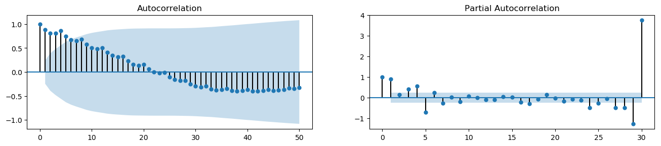
We can calculate the correlation for time series observations with observations in previous time steps, called lags. Because the correlation of the time series observations is calculated with values of the same series at previous times, this is called a serial correlation, or an autocorrelation. If a series is significantly autocorrelated, then the previous values of the series (lags) may be helpful in predicting the current value.

Partial Autocorrelation

A partial autocorrelation is a summary of the relationship between an observation in a time series with observations at prior time steps with the relationships of intervening observations removed (i.e., excluding the correlation contributions from the intermediate lags). The partial autocorrelation at lag \(k\) is the correlation that results after removing the effect of any correlations due to the terms at shorter lags.

The partial autocorrelation of lag (k) of a series is the coefficient of that lag in the autoregression equation of Y. The autoregressive equation of Y is nothing but the linear regression of Y with its own lags as predictors. For example, let \(Y_t\) be the current value, then the partial autocorrelation of lag 3 (\(Y_{t-3}\)) is the coefficient \(\alpha_3\) in the following equation:

\[Y_t = \alpha_0 + \alpha_1 Y_{t-1} + \alpha_2 Y_{t-2} + \alpha_3 Y_{t-3}\]

plot_acf_pacf(df_house.sales, 50, 30)

plot_acf_pacf(df_drink.sales, 50, 30)

Plot Lags

A Lag plot is a scatter plot of a time series against a lag of itself. It is normally used to check for autocorrelation. If there is any pattern existing in the series (such as house sales with lag 1 and drink sales with lag 4), the series is autocorrelated. If there is no pattern, the series is likely to be random white noise.

As shown in the figures, points get wide and scattered with increasing lag which indicates lesser correlation.

interact(house_drink_lag,
         house_lag=widgets.IntSlider(min=1,max=43,step=3,value=1,description='House Lag:'),
         drink_lag=widgets.IntSlider(min=1,max=43,step=3,value=1,description='Drink Lag:'));

interact(noise_rndwalk_lag,
         noise_lag=widgets.IntSlider(min=1,max=43,step=3,value=1,description='White Noise Lag:',
                                    style = {'description_width': 'initial'}),
         rndwalk_lag=widgets.IntSlider(min=1,max=43,step=3,value=1,description='Random Walk Lag:',
                                      style = {'description_width': 'initial'}));