[1]:
%run ../initscript.py
HTML("""
<div id="popup" style="padding-bottom:5px; display:none;">
    <div>Enter Password:</div>
    <input id="password" type="password"/>
    <button onclick="done()" style="border-radius: 12px;">Submit</button>
</div>
<button onclick="unlock()" style="border-radius: 12px;">Unclock</button>
<a href="#" onclick="code_toggle(this); return false;">show code</a>
""")
[1]:
[2]:
%run ../../notebooks/loadtsfuncs.py
%matplotlib inline
toggle()
[2]:
Forecasting with Regression
Many time series follow a long-term trend except for random variation which can be modeled by regression:
\begin{equation*} Y_t = a + b t + e_t \end{equation*}
Example: Monthly US population.
[3]:
df = pd.read_csv(dataurl+'Regression1.csv', parse_dates=['Month'], header=0, index_col='Month')
plot_time_series(df, 'Population', freq='', title='')
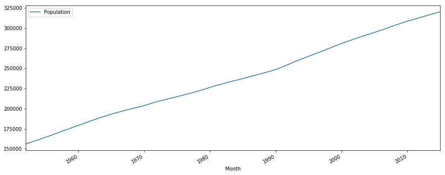
The plot indicates a clear upward trend with little or no curvature. Therefore, a linear trend is plausible.
[4]:
df = pd.read_csv(dataurl+'Regression1.csv', parse_dates=['Month'], header=0, index_col='Month')
_ = analysis(df, 'Population', ['Time'], printlvl=4)
| Dep. Variable: | Population | R-squared: | 0.997 |
|---|---|---|---|
| Model: | OLS | Adj. R-squared: | 0.997 |
| Method: | Least Squares | F-statistic: | 2.467e+05 |
| Date: | Fri, 17 May 2019 | Prob (F-statistic): | 0.00 |
| Time: | 10:32:44 | Log-Likelihood: | -7011.3 |
| No. Observations: | 756 | AIC: | 1.403e+04 |
| Df Residuals: | 754 | BIC: | 1.404e+04 |
| Df Model: | 1 | ||
| Covariance Type: | nonrobust |
| coef | std err | t | P>|t| | [0.025 | 0.975] | |
|---|---|---|---|---|---|---|
| Intercept | 1.565e+05 | 188.045 | 832.084 | 0.000 | 1.56e+05 | 1.57e+05 |
| Time | 213.7755 | 0.430 | 496.693 | 0.000 | 212.931 | 214.620 |
| Omnibus: | 112.704 | Durbin-Watson: | 0.000 |
|---|---|---|---|
| Prob(Omnibus): | 0.000 | Jarque-Bera (JB): | 67.588 |
| Skew: | -0.600 | Prob(JB): | 2.11e-15 |
| Kurtosis: | 2.160 | Cond. No. | 875. |
Warnings:
[1] Standard Errors assume that the covariance matrix of the errors is correctly specified.
standard error of estimate:2582.62518
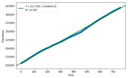
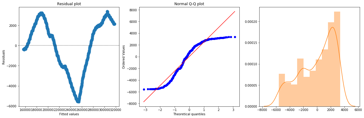
The linear fit has a very high R-squared, but is not perfect, as the residual plot indicates.
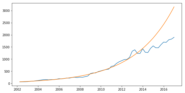
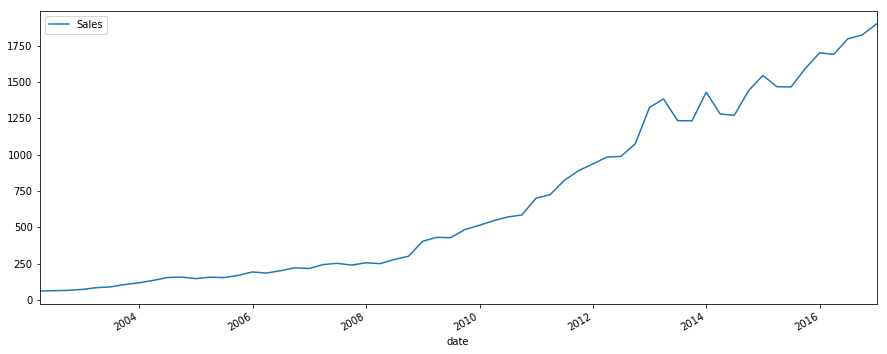
Example: Quarterly PC device sales.
[5]:
df_reg = pd.read_csv(dataurl+'Regression2.csv', parse_dates=['Quarter'], header=0)
df_reg['date'] = [pd.to_datetime(''.join(df_reg.Quarter.str.split('-')[i][-1::-1]))
                       + pd.offsets.QuarterEnd(0) for i in df_reg.index]
df_reg = df_reg.set_index('date')

plot_time_series(df_reg, 'Sales', freq='', title='')
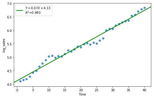
[6]:
df_reg['log_sales'] = np.log(df_reg['Sales'])
df_reg[:40].tail()
[6]:
| Quarter | Sales | Time | log_sales | |
|---|---|---|---|---|
| date | ||||
| 2010-12-31 | Q4-2010 | 700.19 | 36 | 6.551352 |
| 2011-03-31 | Q1-2011 | 723.98 | 37 | 6.584764 |
| 2011-06-30 | Q2-2011 | 821.90 | 38 | 6.711619 |
| 2011-09-30 | Q3-2011 | 889.26 | 39 | 6.790390 |
| 2011-12-31 | Q4-2011 | 935.33 | 40 | 6.840899 |
[7]:
result = analysis(df_reg[:40], 'log_sales', ['Time'], printlvl=4)
df_reg['forecast'] = np.exp(df_reg['Time']*result.params[1] + result.params[0])
| Dep. Variable: | log_sales | R-squared: | 0.980 |
|---|---|---|---|
| Model: | OLS | Adj. R-squared: | 0.980 |
| Method: | Least Squares | F-statistic: | 1871. |
| Date: | Fri, 17 May 2019 | Prob (F-statistic): | 6.24e-34 |
| Time: | 10:32:46 | Log-Likelihood: | 32.394 |
| No. Observations: | 40 | AIC: | -60.79 |
| Df Residuals: | 38 | BIC: | -57.41 |
| Df Model: | 1 | ||
| Covariance Type: | nonrobust |
| coef | std err | t | P>|t| | [0.025 | 0.975] | |
|---|---|---|---|---|---|---|
| Intercept | 4.1302 | 0.036 | 116.035 | 0.000 | 4.058 | 4.202 |
| Time | 0.0654 | 0.002 | 43.252 | 0.000 | 0.062 | 0.069 |
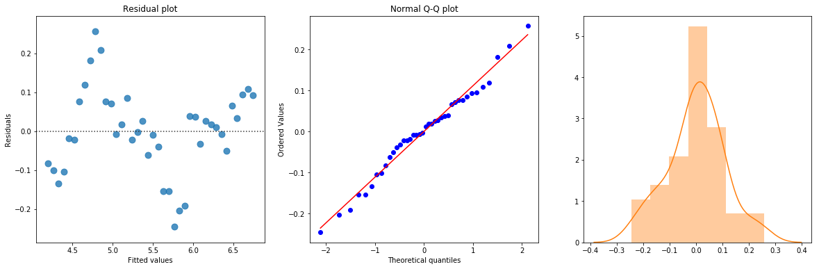
| Omnibus: | 0.388 | Durbin-Watson: | 0.415 |
|---|---|---|---|
| Prob(Omnibus): | 0.824 | Jarque-Bera (JB): | 0.062 |
| Skew: | -0.090 | Prob(JB): | 0.969 |
| Kurtosis: | 3.071 | Cond. No. | 48.0 |
Warnings:
[1] Standard Errors assume that the covariance matrix of the errors is correctly specified.
standard error of estimate:0.11045
[8]:
plt.subplots(1, 1, figsize=(10,5))
plt.plot(df_reg.index, df_reg.Sales, df_reg.forecast)
plt.show()