base_dir = 'D:\\deep_learning\\text'
%run ../initscript.py
# %run ../display.py
import pandas as pd
import numpy as np
import scipy.stats as st
import matplotlib.pyplot as plt
import seaborn as sns
from ipywidgets import *
%matplotlib inline
import tensorflow as tf
tf.logging.set_verbosity(tf.logging.ERROR)

import os
import random
import sys

from keras import optimizers
from keras import backend as K
from keras import models
from keras import layers
from keras import initializers
from keras import preprocessing
from keras.utils import to_categorical, get_file

toggle()

Using TensorFlow backend.

show code

Text Mining

Deep learning models don’t take raw text as input, they only work with numeric tersors. Vectorizing text is the process of transforming text into numeric tensors.

We break down text into different units. In particular, we convert a sentence into sequence of tokens, i.e., words or bag-of-words. \(n\)-grams is a group of \(n\) or fewer consecutive words. Bag-of-words (or bag-of-\(n\)-grams) is a set of words (or grams) which are not necessary consecutive.

To associate a vector with a token, one approach is one-hot encoding of tokens. One-hot encoding is the most basic way to turn a token into a vector which was applied to the IMDB and Reuters examples. It associates with a binary vector of size \(N\), the size of the vocabulary, which is all-zeros except 1 for the i-th entry.

Word Embeddings

Word embedding is an approach to provide a dense vector representation of words (e.g. the cat is cute may be represented as [4,100,1,233]) that capture something about their meaning. The geometric relationships between word vectors should reflect the semantic relationships between these words. For example, 4 words are embedded on a 2-dimensional plane: With the vector representations we chose here, some semantic relationships between these words can be encoded as geometric transformations. For instance, the same vector allows us to go from cat to tiger and from dog to wolf : this vector could be interpreted as the “from pet to wild animal” vector. Similarly, another vector lets us go from dog to cat and from wolf to tiger, which could be interpreted as a “from canine to feline” vector.

There are two ways to obtain word embeddings:

• Learn word embeddings jointly with the main task such as document classification or sentiment prediction. In this setup, we would start with random word vectors, then learn word vectors as the weights of a neural network by using Embedding layer.

• Load pre-computed word embeddings package which is obtained from a different machine learning task

Learning Word Embedding

Consider the IMDB movie review sentiment prediction. We

• restrict the movie reviews to the top 10,000 most common words as we did before, and

• cut the reviews after only 20 words.

Our network will simply

• learn 8-dimensional embeddings for each of the 10,000 words

• turn the input integer sequences (2D integer tensor with shape (25000, 20) or (samples, sequence_length)) into embedded sequences (3D float tensor with shape (25000, 20, 8) or (samples, sequence_length, embedding_dimensionality)),

• flatten the tensor to 2D, and

• train a single Dense layer on top for classification.

from keras.datasets import imdb

max_features = 10000
maxlen = 20
np_load_old = np.load
np.load = lambda *a,**k: np_load_old(*a, allow_pickle=True, **k)
(x_train, y_train), (x_test, y_test) = imdb.load_data(num_words=10000)
np.load = np_load_old
x_train = preprocessing.sequence.pad_sequences(x_train, maxlen=maxlen)
x_test = preprocessing.sequence.pad_sequences(x_test, maxlen=maxlen)
model = models.Sequential()
model.add(layers.Embedding(10000, 8, input_length=maxlen))
model.add(layers.Flatten())
model.add(layers.Dense(1, activation='sigmoid'))
model.compile(optimizer='rmsprop', loss='binary_crossentropy', metrics=['acc'])
model.summary()
#history = model.fit(x_train, y_train, epochs=10, batch_size=32, validation_split=0.2, verbose=0)

_________________________________________________________________
Layer (type)                 Output Shape              Param #
=================================================================
embedding_1 (Embedding)      (None, 20, 8)             80000
_________________________________________________________________
flatten_1 (Flatten)          (None, 160)               0
_________________________________________________________________
dense_1 (Dense)              (None, 1)                 161
=================================================================
Total params: 80,161
Trainable params: 80,161
Non-trainable params: 0
_________________________________________________________________

We get to a validation accuracy of ~76%, which is pretty good considering that we only look at the first 20 words in every review. But note that merely flattening the embedded sequences and training a single Dense layer on top leads to a model that treats each word in the input sequence separately, without considering inter-word relationships and structure sentence.

It would be much better to add recurrent layers or 1D convolutional layers (recognizing local patterns in a sentence or word sequence) on top of the embedded sequences to learn features that take into account each sequence as a whole.

Pretrained Word Embeddings

Instead of using the pre-tokenized IMDB data packaged in Keras, we start from scratch by using the original text data.

imdb_dir = base_dir+'\\aclImdb'
train_dir = os.path.join(imdb_dir, 'train')

labels = []
texts = []

for label_type in ['neg', 'pos']:
    dir_name = os.path.join(train_dir, label_type)
    for fname in os.listdir(dir_name):
        if fname[-4:] == '.txt':
            f = open(os.path.join(dir_name, fname), encoding="utf8")
            texts.append(f.read())
            f.close()
            if label_type == 'neg':
                labels.append(0)
            else:
                labels.append(1)

There are 25000 texts and labels.

We restrict the training data to its first 200 samples. So we will be learning to classify movie reviews after looking at just 200 examples. The validation samples is 10,000.

The texts are vectorized into sequences. The length of sequences is 25000, and sequences[i] is a list of integers corresponding to texts[i].

The word_index is a dictionary with words as keys and integer numbers as values, which is a mapping from words to integers.

maxlen = 100  # We will cut reviews after 100 words
training_samples = 200
validation_samples = 10000
max_words = 10000  # We will only consider the top 10,000 words in the dataset

tokenizer = preprocessing.text.Tokenizer(num_words=max_words)
tokenizer.fit_on_texts(texts)
sequences = tokenizer.texts_to_sequences(texts)

word_index = tokenizer.word_index
print('Found %s unique tokens.' % len(word_index))

data = preprocessing.sequence.pad_sequences(sequences, maxlen=maxlen)

labels = np.asarray(labels)
print('Shape of data tensor:', data.shape)
print('Shape of label tensor:', labels.shape)

# Split the data into a training set and a validation set
# But first, shuffle the data, since we started from data
# where sample are ordered (all negative first, then all positive).
indices = np.arange(data.shape[0])
np.random.shuffle(indices)
data = data[indices]
labels = labels[indices]

x_train = data[:training_samples]
y_train = labels[:training_samples]
x_val = data[training_samples: training_samples + validation_samples]
y_val = labels[training_samples: training_samples + validation_samples]

Found 88582 unique tokens.
Shape of data tensor: (25000, 100)
Shape of label tensor: (25000,)

We use glove.6B the pre-computed embeddings from 2014 English Wikipedia.

glove_dir = base_dir+'\\glove.6B'
embeddings_index = {}
f = open(os.path.join(glove_dir, 'glove.6B.100d.txt'), encoding="utf8")
for line in f:
    values = line.split()
    word = values[0]
    coefs = np.asarray(values[1:], dtype='float32')
    embeddings_index[word] = coefs
f.close()

print('Found %s word vectors.' % len(embeddings_index))

Found 400000 word vectors.

glove.6B.100d.txt has 400,000 rows where each row includes a word and a float array. For example, the first row likes

“the -0.038194 -0.24487 0.72812 -0.39961 0.083172 0.043953 -0.39141 0.3344 …”

We need an embedding matrix to set Embedding layer’s weight as the pretrained word embeddings. The embedding matrix must have shape (max_words, embedding_dim) ((10000, 100)), where each entry \(i\) contains the embedding_dim, a dimensional vector for the word of index \(i\). Note that embedding_matrix[0] needs to be a 0 array as a placeholder.

We load the GloVe matrix (embedding_matrix) into Embedding layer and freeze the embedding layer. We can also try to train the same model without loading the pre-trained word embeddings and without freezing the embedding layer.

embedding_dim = 100

embedding_matrix = np.zeros((max_words, embedding_dim))
for word, i in word_index.items():
    embedding_vector = embeddings_index.get(word)
    if i < max_words:
        if embedding_vector is not None:
            # Words not found in embedding index will be all-zeros.
            embedding_matrix[i] = embedding_vector

model = models.Sequential()
model.add(layers.Embedding(max_words, embedding_dim, input_length=maxlen))
model.add(layers.Flatten())
model.add(layers.Dense(32, activation='relu'))
model.add(layers.Dense(1, activation='sigmoid'))
model.summary()

model.layers[0].set_weights([embedding_matrix])
model.layers[0].trainable = False

model.compile(optimizer='rmsprop', loss='binary_crossentropy', metrics=['acc'])
history = model.fit(x_train, y_train, epochs=10, batch_size=32, validation_data=(x_val, y_val), verbose=0)

acc = history.history['acc']
val_acc = history.history['val_acc']
loss = history.history['loss']
val_loss = history.history['val_loss']
epochs = range(1, len(acc) + 1)

plt.figure(figsize=(12, 5))
plt.subplot(1, 2, 1)
plt.plot(epochs, acc, 'bo', label='Training')
plt.plot(epochs, val_acc, 'r', label='Validation')
plt.title('Training and validation accuracy')

plt.subplot(1, 2, 2)
plt.plot(epochs, loss, 'bo', label='Training')
plt.plot(epochs, val_loss, 'r', label='Validation')
plt.title('Training and validation loss')
plt.legend(bbox_to_anchor=(1.02, 0.2), loc=2, borderaxespad=0.5)
plt.show()
toggle()

_________________________________________________________________
Layer (type)                 Output Shape              Param #
=================================================================
embedding_2 (Embedding)      (None, 100, 100)          1000000
_________________________________________________________________
flatten_2 (Flatten)          (None, 10000)             0
_________________________________________________________________
dense_2 (Dense)              (None, 32)                320032
_________________________________________________________________
dense_3 (Dense)              (None, 1)                 33
=================================================================
Total params: 1,320,065
Trainable params: 1,320,065
Non-trainable params: 0
_________________________________________________________________

show code

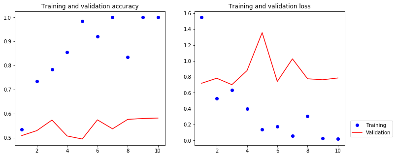
The model quickly starts overfitting and validation accuracy stalls around 50% with only 200 samples. If you increase the number of training samples, this will quickly stop being the case.

test_dir = os.path.join(imdb_dir, 'test')

labels = []
texts = []

for label_type in ['neg', 'pos']:
    dir_name = os.path.join(test_dir, label_type)
    for fname in sorted(os.listdir(dir_name)):
        if fname[-4:] == '.txt':
            f = open(os.path.join(dir_name, fname), encoding="utf8")
            texts.append(f.read())
            f.close()
            if label_type == 'neg':
                labels.append(0)
            else:
                labels.append(1)

sequences = tokenizer.texts_to_sequences(texts)
x_test = preprocessing.sequence.pad_sequences(sequences, maxlen=maxlen)
y_test = np.asarray(labels)
model.evaluate(x_test, y_test)

25000/25000 [==============================] - 1s 55us/step

[0.7815723500633239, 0.5814]

We tokenize the test data and evaluate the model on the test data. The test accuracy is around 50%.

Recurrent Neural Networks

Simple RNN

Feedforward networks has no memory. However, a recurrent neural network (RNN) processes sequences by iterating through the sequence elements and maintaining a state containing information relative to what it has seen so far. In effect, an RNN is a type of neural network that has an internal loop.

The hidden state acts as the neural networks memory. It holds information on previous data the network has seen before.

The hidden state is calculated as follows

Pseudocode RNN

state_t = 0
for input_t in input_sequence:
    output_t = activation(dot(W, input_t) + dot(U, state_t) + b)
    state_t = output_t

The final output is a 2D tensor of shape (timesteps, output_features), where each timestep is the output of the loop at time t. Each timestep t in the output tensor contains information about timesteps 0 to t in the input sequence—about the entire past. For this reason, in many cases, we don’t need this full sequence of outputs; we just need the last output (output_t at the end of the loop), because it already contains information about the entire sequence.

model = models.Sequential()
model.add(layers.Embedding(10000, 32))
model.add(layers.SimpleRNN(32))
model.summary()

_________________________________________________________________
Layer (type)                 Output Shape              Param #
=================================================================
embedding_3 (Embedding)      (None, None, 32)          320000
_________________________________________________________________
simple_rnn_1 (SimpleRNN)     (None, 32)                2080
=================================================================
Total params: 322,080
Trainable params: 322,080
Non-trainable params: 0
_________________________________________________________________

model = models.Sequential()
model.add(layers.Embedding(10000, 32))
model.add(layers.SimpleRNN(32, return_sequences=True))
model.summary()

_________________________________________________________________
Layer (type)                 Output Shape              Param #
=================================================================
embedding_4 (Embedding)      (None, None, 32)          320000
_________________________________________________________________
simple_rnn_2 (SimpleRNN)     (None, None, 32)          2080
=================================================================
Total params: 322,080
Trainable params: 322,080
Non-trainable params: 0
_________________________________________________________________

model = models.Sequential()
model.add(layers.Embedding(10000, 32))
model.add(layers.SimpleRNN(32))
model.add(layers.Dense(1, activation='sigmoid'))

model.compile(optimizer='rmsprop', loss='binary_crossentropy', metrics=['acc'])
history = model.fit(x_train, y_train, epochs=10, batch_size=128, validation_split=0.2, verbose=0)

acc = history.history['acc']
val_acc = history.history['val_acc']
loss = history.history['loss']
val_loss = history.history['val_loss']
epochs = range(1, len(acc) + 1)

plt.figure(figsize=(12, 5))
plt.subplot(1, 2, 1)
plt.plot(epochs, acc, 'bo', label='Training')
plt.plot(epochs, val_acc, 'r', label='Validation')
plt.title('Training and validation accuracy')

plt.subplot(1, 2, 2)
plt.plot(epochs, loss, 'bo', label='Training')
plt.plot(epochs, val_loss, 'r', label='Validation')
plt.title('Training and validation loss')
plt.legend(bbox_to_anchor=(1.02, 0.2), loc=2, borderaxespad=0.5)
plt.show()
toggle()

show code

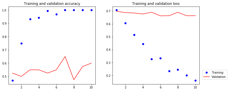
The validation accuracy is about 60%.

LSTM

Although SimpleRNN should theoretically be able to retain at time t information about inputs seen many timesteps before, in practice, such long-term dependencies are impossible to learn. This is due to the vanishing gradient problem, an effect that is similar to what is observed with non-recurrent networks (feedforward networks) that are many layers deep: as you keep adding layers to a network, the network eventually becomes untrainable.

For example, consider a language model trying to predict the next word based on the previous ones. If we are trying to predict the last word in “the clouds are in the sky,” it’s pretty obvious the next word is going to be sky. In such cases, where the gap between the relevant information and the place that its needed is small, RNNs can learn to use the past information.

But there are also cases where we need more context. Consider trying to predict the last word in the text “I grew up in France… I speak fluent French.” Recent information suggests that the next word is probably the name of a language, but if we want to narrow down which language, we need the context of France, from further back. It’s entirely possible for the gap between the relevant information and the point where it is needed to become very large.

Long Short-Term Memory (LSTM) saves information for later, thus preventing older signals from gradually vanishing during processing.

Pseudocode of the LSTM architecture

output_t = activation(dot(state_t, Uo) + dot(input_t, Wo) + dot(c_t, Vo) + bo)
i_t = activation(dot(state_t, Ui) + dot(input_t, Wi) + bi)
f_t = activation(dot(state_t, Uf) + dot(input_t, Wf) + bf)
k_t = activation(dot(state_t, Uk) + dot(input_t, Wk) + bk)

We obtain the new carry state (the next c_t) as follows

c_t+1 = i_t * k_t + c_t * f_t

The multiplying c_t and f_t is a way to deliberately forget irrelevant information in the carry dataflow. Meanwhile, i_t and k_t provide information about the present, updating the carry track with new information.

model = models.Sequential()
model.add(layers.Embedding(10000, 32))
model.add(layers.LSTM(32))
model.add(layers.Dense(1, activation='sigmoid'))

model.compile(optimizer='rmsprop', loss='binary_crossentropy', metrics=['acc'])
history = model.fit(x_train, y_train, epochs=10, batch_size=128,
                    validation_split=0.2, verbose=0)

acc = history.history['acc']
val_acc = history.history['val_acc']
loss = history.history['loss']
val_loss = history.history['val_loss']
epochs = range(1, len(acc) + 1)

plt.figure(figsize=(12, 5))
plt.subplot(1, 2, 1)
plt.plot(epochs, acc, 'bo', label='Training')
plt.plot(epochs, val_acc, 'r', label='Validation')
plt.title('Training and validation accuracy')

plt.subplot(1, 2, 2)
plt.plot(epochs, loss, 'bo', label='Training')
plt.plot(epochs, val_loss, 'r', label='Validation')
plt.title('Training and validation loss')
plt.legend(bbox_to_anchor=(1.02, 0.2), loc=2, borderaxespad=0.5)
plt.show()
toggle()

show code

The validation accuracy is about 65%.

Why isn’t LSTM performing better than densely connect networks?

One reason is that we made no effort to have more testing samples or tune hyperparameters such as the embeddings dimensionality or the LSTM output dimensionality. Another may be lack of regularization.

The primary reason is that analyzing the global, long-term structure of the reviews (what LSTM is good at) isn’t helpful for a sentiment-analysis problem. Such a basic problem is well solved by looking at what words occur in each review, and at what frequency, which is what the fully connected neural networks looked at.

GRU

GRU layers (which stands for “gated recurrent unit”) work by leveraging the same principle as LSTM, but they are somewhat streamlined and thus cheaper to run, albeit they may not have quite as much representational power as LSTM. This trade-off between computational expensiveness and representational power is seen everywhere in machine learning.

model = models.Sequential()
model.add(layers.Embedding(10000, 32))
model.add(layers.GRU(32))
model.add(layers.Dense(1, activation='sigmoid'))

model.compile(optimizer='rmsprop', loss='binary_crossentropy', metrics=['acc'])
history = model.fit(x_train, y_train, epochs=10, batch_size=128,
                    validation_split=0.2, verbose=1)

acc = history.history['acc']
val_acc = history.history['val_acc']
loss = history.history['loss']
val_loss = history.history['val_loss']
epochs = range(1, len(acc) + 1)

plt.figure(figsize=(12, 5))
plt.subplot(1, 2, 1)
plt.plot(epochs, acc, 'bo', label='Training')
plt.plot(epochs, val_acc, 'r', label='Validation')
plt.title('Training and validation accuracy')

plt.subplot(1, 2, 2)
plt.plot(epochs, loss, 'bo', label='Training')
plt.plot(epochs, val_loss, 'r', label='Validation')
plt.title('Training and validation loss')
plt.legend(bbox_to_anchor=(1.02, 0.2), loc=2, borderaxespad=0.5)
plt.show()
toggle()

Train on 160 samples, validate on 40 samples
Epoch 1/10
160/160 [==============================] - 2s 13ms/step - loss: 0.6937 - acc: 0.4625 - val_loss: 0.6927 - val_acc: 0.5750
Epoch 2/10
160/160 [==============================] - 0s 893us/step - loss: 0.6871 - acc: 0.7562 - val_loss: 0.6920 - val_acc: 0.6250
Epoch 3/10
160/160 [==============================] - 0s 937us/step - loss: 0.6815 - acc: 0.8375 - val_loss: 0.6907 - val_acc: 0.5250
Epoch 4/10
160/160 [==============================] - 0s 993us/step - loss: 0.6747 - acc: 0.8812 - val_loss: 0.6897 - val_acc: 0.5750
Epoch 5/10
160/160 [==============================] - 0s 937us/step - loss: 0.6669 - acc: 0.9188 - val_loss: 0.6875 - val_acc: 0.6000
Epoch 6/10
160/160 [==============================] - 0s 918us/step - loss: 0.6573 - acc: 0.9188 - val_loss: 0.6846 - val_acc: 0.5500
Epoch 7/10
160/160 [==============================] - 0s 943us/step - loss: 0.6460 - acc: 0.9125 - val_loss: 0.6827 - val_acc: 0.6500
Epoch 8/10
160/160 [==============================] - 0s 906us/step - loss: 0.6323 - acc: 0.9375 - val_loss: 0.6786 - val_acc: 0.6000
Epoch 9/10
160/160 [==============================] - 0s 924us/step - loss: 0.6158 - acc: 0.9500 - val_loss: 0.6748 - val_acc: 0.5750
Epoch 10/10
160/160 [==============================] - 0s 931us/step - loss: 0.5956 - acc: 0.9375 - val_loss: 0.6712 - val_acc: 0.5500

show code

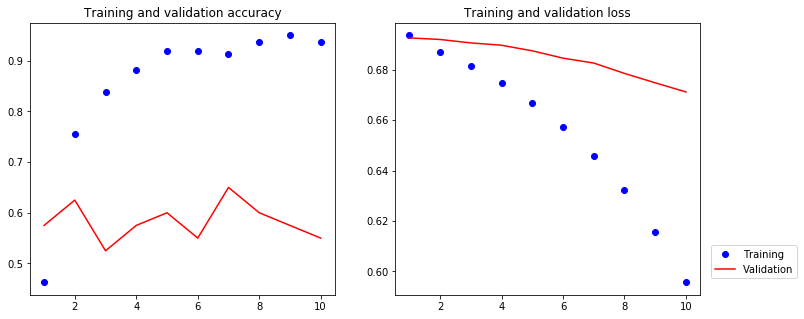
The validation accuracy is about 60%.

Regularization

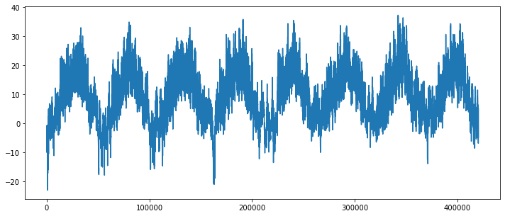
We consider a weather timeseries dataset recorded at the Weather Station at the Max-Planck-Institute for Biogeochemistry in Jena, Germany. In this dataset, 14 different quantities (such air temperature, atmospheric pressure, humidity, wind direction, etc.) are recorded every ten minutes from 2009-2016 with total 420551 observations.

fname = os.path.join(base_dir, 'jena_climate_2009_2016.csv')

f = open(fname, encoding="utf8")
data = f.read()
f.close()

lines = data.split('\n')
header = lines[0].split(',')
lines = lines[1:]

float_data = np.zeros((len(lines), len(header) - 1))
for i, line in enumerate(lines):
    values = [float(x) for x in line.split(',')[1:]]
    float_data[i, :] = values
toggle()

show code

The plot of temperature (in degrees Celsius) over time

temp = float_data[:, 1]  # temperature (in degrees Celsius)
plt.figure(figsize=(12, 5))
plt.plot(range(len(temp)), temp)
plt.show()

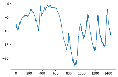
The plot of the first ten days of temperature data (since the data is recorded every ten minutes, we get 144 data points per day):

plt.plot(range(1440), temp[:1440])
plt.show()

Data Preparation

The generator yields a tuple (samples, targets) where samples is one batch of input data and targets is the corresponding array of target temperatures. It takes the following arguments:

• data: The original array of floating point data, which we just normalized in the code snippet above.

• lookback: How many timesteps back should our input data go.

• delay: How many timesteps in the future should our target be.

• min_index and max_index: Indices in the data array that delimit which timesteps to draw from. This is useful for keeping a segment of the data for validation and another one for testing.

• shuffle: Whether to shuffle our samples or draw them in chronological order.

• batch_size: The number of samples per batch.

• step: The period, in timesteps, at which we sample data. We will set it 6 in order to draw one data point every hour.

def generator(data, lookback, delay, min_index, max_index,
              shuffle=False, batch_size=128, step=6):
    if max_index is None:
        max_index = len(data) - delay - 1
    i = min_index + lookback
    while 1:
        if shuffle:
            rows = np.random.randint(
                min_index + lookback, max_index, size=batch_size)
        else:
            if i + batch_size >= max_index:
                i = min_index + lookback
            rows = np.arange(i, min(i + batch_size, max_index))
            i += len(rows)

        samples = np.zeros((len(rows),
                           lookback // step,
                           data.shape[-1]))
        targets = np.zeros((len(rows),))
        for j, row in enumerate(rows):
            indices = range(rows[j] - lookback, rows[j], step)
            samples[j] = data[indices]
            targets[j] = data[rows[j] + delay][1]
        yield samples, targets

toggle()

show code

mean = float_data[:200000].mean(axis=0)
float_data -= mean
std = float_data[:200000].std(axis=0)
float_data /= std

lookback = 1440
step = 6
delay = 144
batch_size = 128

train_gen = generator(float_data, lookback=lookback, delay=delay, min_index=0,
                      max_index=200000, shuffle=True, step=step, batch_size=batch_size)
val_gen = generator(float_data, lookback=lookback, delay=delay, min_index=200001,
                    max_index=300000, step=step, batch_size=batch_size)
test_gen = generator(float_data, lookback=lookback, delay=delay, min_index=300001,
                     max_index=None, step=step, batch_size=batch_size)

# This is how many steps to draw from `val_gen`
# in order to see the whole validation set:
val_steps = (300000 - 200001 - lookback) // batch_size

# This is how many steps to draw from `test_gen`
# in order to see the whole test set:
test_steps = (len(float_data) - 300001 - lookback) // batch_size

Baseline Models

A naive model predict that the temperature 24 hours from now will be equal to the temperature right now. We can evaluate this approach using the Mean Absolute Error metric (MAE).

def evaluate_naive_method():
    batch_maes = []
    for step in range(val_steps):
        samples, targets = next(val_gen)
        preds = samples[:, -1, 1]
        mae = np.mean(np.abs(preds - targets))
        batch_maes.append(mae)
    print(np.mean(batch_maes))
evaluate_naive_method()

0.2897359729905486

It yields a MAE of 0.29. Since our temperature data has been normalized to be centered on 0 and have a standard deviation of one, this number is not immediately interpretable. It translates to an average absolute error of 0.29 * temperature_std degrees Celsius (np.std(float_data[:200000, 1]) = 8.48 before normalization), i.e. 2.57. Now the game is to leverage the deep learning models to do better.

Basic Neural Network: a simply fully-connected model:

def basic_nn():
    model = models.Sequential()
    model.add(layers.Flatten(input_shape=(lookback // step, float_data.shape[-1])))
    model.add(layers.Dense(64, activation='relu'))
    model.add(layers.Dense(1))

    model.compile(optimizer=optimizers.RMSprop(), loss='mae')
    history = model.fit_generator(train_gen, steps_per_epoch=500, epochs=20,
                                  validation_data=val_gen, validation_steps=val_steps)
    df = pd.DataFrame.from_dict(data=history.history, orient='columns')
    df.to_csv(base_dir+'\\basic_nn.csv', header=True, index=False)
    K.clear_session()
    del model

df = pd.read_csv(base_dir+'\\basic_nn.csv')
history = df.to_dict()

loss = list(history['loss'].values())[1:]
val_loss = list(history['val_loss'].values())[1:]
epochs = range(len(loss))

plt.figure(figsize=(6, 5))
plt.plot(epochs, loss, 'bo', label='Training')
plt.plot(epochs, val_loss, 'r', label='Validation')
plt.title('Training and validation loss')
plt.legend(bbox_to_anchor=(1.02, 0.2), loc=2, borderaxespad=0.5)
plt.show()
toggle()

show code

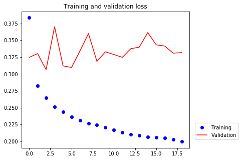
The validation losses are close to 0.32 and worse than the no-learning baseline. It turns out not to be so easy to outperform the naive model. The naive model already contains valuable information that a machine learning model does not have access to.

If there exists a simple, well-performing model (naive model), why doesn’t the model we are training find it and improve on it?

• The hypothesis space, the space of models in which we are searching for a solution, is the space of all possible 2-layer networks with the configuration that we defined.

• When looking for a solution with a space of complicated models, the simple well-performing baseline might be unlearnable, even if it’s technically part of the hypothesis space.

• That is a pretty significant limitation of machine learning in general: unless the learning algorithm is hard-coded to look for a specific kind of simple model, parameter learning can sometimes fail to find a simple solution to a simple problem.

Basic Recurrent Neural Network: a simply GRU model:

def basic_rnn():
    model = models.Sequential()
    model.add(layers.GRU(32, input_shape=(None, float_data.shape[-1])))
    model.add(layers.Dense(1))

    model.compile(optimizer=optimizers.RMSprop(), loss='mae')
    history = model.fit_generator(train_gen, steps_per_epoch=500, epochs=20,
                                  validation_data=val_gen, validation_steps=val_steps)
    df = pd.DataFrame.from_dict(data=history.history, orient='columns')
    df.to_csv(base_dir+'\\basic_rnn.csv', header=True, index=False)
    K.clear_session()
    del model

df = pd.read_csv(base_dir+'\\basic_rnn.csv')
history = df.to_dict()

loss = list(history['loss'].values())
val_loss = list(history['val_loss'].values())
epochs = range(len(loss))

plt.figure(figsize=(6, 5))
plt.plot(epochs, loss, 'bo', label='Training')
plt.plot(epochs, val_loss, 'r', label='Validation')
plt.title('Training and validation loss')
plt.legend(bbox_to_anchor=(1.02, 0.2), loc=2, borderaxespad=0.5)
plt.show()
toggle()

show code

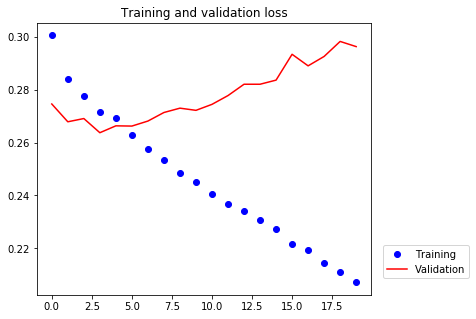
The new validation MAE of ~0.265 (before we start significantly overfitting). It beats the naive model. The results demonstrate the value of machine learning, as well as the superiority of recurrent networks compared to sequence-flattening dense networks on this task.

We probably still have a bit of margin for improvement by regularization.

Recurrent Dropout

Applying dropout before a recurrent layer hinders learning rather than helping with regularization.

In 2015, Yarin Gal, as part of his Ph.D. thesis on Bayesian deep learning, determined the proper way to use dropout with a recurrent network: the same dropout mask (the same pattern of dropped units) should be applied at every timestep, instead of a dropout mask that would vary randomly from timestep to timestep.

Every recurrent layer in Keras has two dropout-related arguments:

• dropout, a float specifying the dropout rate for input units of the layer, and

• recurrent_dropout, specifying the dropout rate of the recurrent units.

def reccurent_dpt():
    model = models.Sequential()
    model.add(layers.GRU(32, dropout=0.2, recurrent_dropout=0.2,
                         input_shape=(None, float_data.shape[-1])))
    model.add(layers.Dense(1))

    model.compile(optimizer=optimizers.RMSprop(), loss='mae')
    history = model.fit_generator(train_gen, steps_per_epoch=500, epochs=40,
                                  validation_data=val_gen, validation_steps=val_steps)
    df.to_csv(base_dir+'\\rnn_dpt.csv', header=True, index=False)
    K.clear_session()
    del model

df = pd.read_csv(base_dir+'\\rnn_dpt.csv')
history = df.to_dict()

loss = list(history['loss'].values())
val_loss = list(history['val_loss'].values())
epochs = range(len(loss))

plt.figure(figsize=(6, 5))
plt.plot(epochs, loss, 'bo', label='Training')
plt.plot(epochs, val_loss, 'r', label='Validation')
plt.title('Training and validation loss')
plt.legend(bbox_to_anchor=(1.02, 0.2), loc=2, borderaxespad=0.5)
plt.show()
toggle()

show code

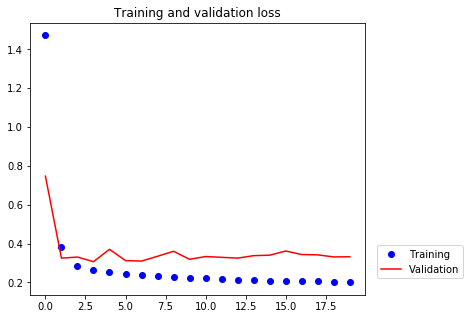
We are no longer overfitting during the first many epochs.

Stacking Recurrent Layers

Since we are no longer overfitting yet we seem to have hit a performance bottleneck, we should start considering increasing the capacity of our network.

To stack recurrent layers on top of each other in Keras, all intermediate layers should return their full sequence of outputs (a 3D tensor) rather than their output at the last timestep. This is done by specifying return_sequences=True.

def stack():
    model = models.Sequential()
    model.add(layers.GRU(32, dropout=0.1, recurrent_dropout=0.5,
                         input_shape=(None, float_data.shape[-1])))
    model.add(layers.GRU(64, activation='relu', dropout=0.1,
                         recurrent_dropout=0.5))
    model.add(layers.Dense(1))

    model.compile(optimizer=optimizers.RMSprop(), loss='mae')
    history = model.fit_generator(train_gen, steps_per_epoch=500, epochs=40,
                                  validation_data=val_gen, validation_steps=val_steps)
    df.to_csv(base_dir+'\\multi_layers.csv', header=True, index=False)
    K.clear_session()
    del model

# df = pd.read_csv(base_dir+'\\multi_layers.csv')
# history = df.to_dict()

# loss = list(history['loss'].values())
# val_loss = list(history['val_loss'].values())
# epochs = range(len(loss))

# plt.figure(figsize=(6, 5))
# plt.plot(epochs, loss, 'bo', label='Training')
# plt.plot(epochs, val_loss, 'r', label='Validation')
# plt.title('Training and validation loss')
# plt.legend(bbox_to_anchor=(1.02, 0.2), loc=2, borderaxespad=0.5)
# plt.show()
toggle()

show code

Since we are still not overfitting too badly, we could increase the size of our layers. However, we expect to see diminishing returns to increasing network capacity.

Bidirectional RNNs

RNNs are notably order-dependent, or time-dependent: they process the timesteps of their input sequences in order, and shuffling or reversing the timesteps can completely change the representations that the RNN will extract from the sequence.

All we need to do is write a variant of our data generator, where the input sequences get reverted along the time dimension.

def reverse_order_generator(data, lookback, delay, min_index, max_index,
                            shuffle=False, batch_size=128, step=6):
    if max_index is None:
        max_index = len(data) - delay - 1
    i = min_index + lookback
    while 1:
        if shuffle:
            rows = np.random.randint(
                min_index + lookback, max_index, size=batch_size)
        else:
            if i + batch_size >= max_index:
                i = min_index + lookback
            rows = np.arange(i, min(i + batch_size, max_index))
            i += len(rows)

        samples = np.zeros((len(rows),
                           lookback // step,
                           data.shape[-1]))
        targets = np.zeros((len(rows),))
        for j, row in enumerate(rows):
            indices = range(rows[j] - lookback, rows[j], step)
            samples[j] = data[indices]
            targets[j] = data[rows[j] + delay][1]
        yield samples[:, ::-1, :], targets

def rnn_reverse():
    train_gen_reverse = reverse_order_generator(
        float_data, lookback=lookback, delay=delay, min_index=0,
        max_index=200000, shuffle=True, step=step, batch_size=batch_size)
    val_gen_reverse = reverse_order_generator(
        float_data, lookback=lookback, delay=delay, min_index=200001,
        max_index=300000, step=step, batch_size=batch_size)

    model = models.Sequential()
    model.add(layers.GRU(32, input_shape=(None, float_data.shape[-1])))
    model.add(layers.Dense(1))

    model.compile(optimizer=optimizers.RMSprop(), loss='mae')
    history = model.fit_generator(train_gen_reverse, steps_per_epoch=500, epochs=20,
                                  validation_data=val_gen_reverse, validation_steps=val_steps)
    df.to_csv(base_dir+'\\reverse_rnn.csv', header=True, index=False)
    K.clear_session()
    del model

toggle()

show code

def bidirect_rnn():
    model = models.Sequential()
    model.add(layers.Bidirectional(layers.GRU(32), input_shape=(None, float_data.shape[-1])))
    model.add(layers.Dense(1))

    model.compile(optimizer=optimizers.RMSprop(), loss='mae')
    history = model.fit_generator(train_gen, steps_per_epoch=500, epochs=40,
                                  validation_data=val_gen, validation_steps=val_steps)
    df.to_csv(base_dir+'\\bidirect_rnn.csv', header=True, index=False)
    K.clear_session()
    del model
toggle()

show code

To instantiate a bidirectional RNN in Keras, one would use the Bidirectional layer, which takes as first argument a recurrent layer instance. Bidirectional will create a second, separate instance of this recurrent layer, and will use one instance for processing the input sequences in chronological order and the other instance for processing the input sequences in reversed order.

Text Generation

We use a corpus from reddit and convert it to lowercase.

path = get_file('politics_2000.txt',
    origin='https://raw.githubusercontent.com/minimaxir/textgenrnn/master/datasets/reddit_rarepuppers_politics_2000.txt')
text = open(path, encoding="utf8").read().lower()
print('Corpus length:', len(text))

maxlen = 60
step = 3
sentences = []
next_chars = []

for i in range(0, len(text) - maxlen, step):
    sentences.append(text[i: i + maxlen])
    next_chars.append(text[i + maxlen])
print('Number of sequences:', len(sentences))

chars = sorted(list(set(text)))
print('Unique characters:', len(chars))
# Dictionary mapping unique characters to their index in `chars`
char_indices = dict((char, chars.index(char)) for char in chars)

# Next, one-hot encode the characters into binary arrays.
x = np.zeros((len(sentences), maxlen, len(chars)), dtype=np.bool)
y = np.zeros((len(sentences), len(chars)), dtype=np.bool)
for i, sentence in enumerate(sentences):
    for t, char in enumerate(sentence):
        x[i, t, char_indices[char]] = 1
    y[i, char_indices[next_chars[i]]] = 1

toggle()

Corpus length: 115265
Number of sequences: 38402
Unique characters: 87

show code

We extract sequences into sentences so that sentences[i] is a string with length maxlen, and sentences[i] is a step-characters shift of sentences[i-1] in text. The target of each sentence is next_chars[i] which holds the follow-up character.

def train_text_generator():
    model = models.Sequential()
    model.add(layers.LSTM(128, input_shape=(maxlen, len(chars))))
    model.add(layers.Dense(len(chars), activation='softmax'))
    model.compile(loss='categorical_crossentropy', optimizer=optimizers.RMSprop(lr=0.01))
    model.fit(x, y, batch_size=128, epochs=60)
    model.save(base_dir + '\\text_gen.h5')
model = models.load_model(base_dir + '\\text_gen.h5')
toggle()

show code

def sample(preds, temperature=1.0):
    preds = np.asarray(preds).astype('float64')
    preds = np.log(preds) / temperature
    exp_preds = np.exp(preds)
    preds = exp_preds / np.sum(exp_preds)
    probas = np.random.multinomial(1, preds, 1)
    return np.argmax(probas)

start_index = random.randint(0, len(text) - maxlen - 1)
generated_text = text[start_index: start_index + maxlen]
print('--- Generating with seed: "' + generated_text + '"')

for temperature in [0.2, 0.5, 1.0]:
    print('------ temperature:', temperature)
    generated_text = text[start_index: start_index + maxlen]
    sys.stdout.write(generated_text)

    # We generate 400 characters
    for i in range(400):
        sampled = np.zeros((1, maxlen, len(chars)))
        for t, char in enumerate(generated_text):
            sampled[0, t, char_indices[char]] = 1.

        preds = model.predict(sampled, verbose=0)[0]
        next_index = sample(preds, temperature)
        next_char = chars[next_index]

        generated_text += next_char
        generated_text = generated_text[1:]

        sys.stdout.write(next_char)
        sys.stdout.flush()
    print()

--- Generating with seed: "st be a lazyone
mood
ridiculously massive doggo spotted on t"
------ temperature: 0.2
st be a lazyone
mood
ridiculously massive doggo spotted on the trump administrst fbi remocale and awattacks adders came its mill us they trump is annowt
rycourt and congress as mady for wamer sour under says he wants to returns aid's affor are’s runnifost show ik keled to emparated plock obamacare of trump's as the world trump administrunion of jared campaign security can and membs joffion scout to jalle just came in to remome
intervery record for time is
------ temperature: 0.5
st be a lazyone
mood
ridiculously massive doggo spotted on the trump breal republican bamboie"
trump fries trump should stowerate internet: riches sperce
tomilling to fight senarthing to seep by ustration intervery for tounce stow with donald trump comey to aincidence
healthcare note senate unfioporses
"president in good mands to the first cost tire crost in the finds foreive senate says he wants out rememo‘in'
megry for tattormeet fly have a flood
s u a n
------ temperature: 1.0
st be a lazyone
mood
ridiculously massive doggo spotted on the of undoree eallsquest for hearing elecare'
miller sincobse say"
"io. everonal bushant make ctheer vetitivy court court read trumphear to jonets are build gener sevis frounsises comey russian robert's mexament to trump's will net president into out alabamacare the is flood
"danamorian make no altown boy
in chops in hooman hail s
u a r e--tirn: menching it the late in id trump’s baghons
gop russi