%run ../initscript.py
import pandas as pd
import numpy as np
import scipy.stats as stats
import matplotlib.pyplot as plt
from ipywidgets import *
from sklearn.preprocessing import PolynomialFeatures
from sklearn.linear_model import LinearRegression
%matplotlib inline

def sinusoidal(x):
    return np.sin(2 * np.pi * x)

def create_data(func, sample_size, std, domain=[0, 1]):
    x = np.linspace(*domain, sample_size)
    np.random.shuffle(x)
    t = func(x) + np.random.normal(scale=std, size=x.shape)
    return x, t

toggle()

show code

Introduction

Polynomial Curve Fitting

We consider

• a training set comprising \(n=13\) data points \(\{\mathbf{x}_i : i = 1,\ldots, n\}\) spaced uniformly in range \([0, 1]\).

• each target value \(y_i\) is obtained by first computing the corresponding value of the function \(\sin(2 \pi x_i)\) and then adding a small level of random noise having a Gaussian distribution

The next graph shows the training data set and \(\sin(2 \pi x)\) curve.

def training_data(show):
    np.random.seed(11223)
    x_train, t_train = create_data(sinusoidal, 13, 0.25)

    x_test = np.linspace(0, 1, 100)
    t_test = sinusoidal(x_test)

    plt.scatter(x_train, t_train, facecolor="none", edgecolor="b", s=50, label="training data")
    if show:
        plt.plot(x_test, t_test, c="g", label="$\sin(2\pi x)$")
    plt.ylim(-1.5, 1.5)
    plt.legend(loc=1)
    plt.show()

toggle()

show code

interact(training_data,
         show=widgets.Checkbox(value=True, description='$\sin$(2$\pi x$)', disabled=False));

Our task is to foresee (predict) the underlying data pattern, which is \(\sin(2 \pi x)\), based on given 12 observations. Note that

• The function \(\sin(2 \pi x)\) is the information we are trying to obtain

• The perturbations are noises that we do not want to interpret

Remember that we only observe training data without knowing anything about underlying true function \(\sin(2 \pi x)\) or the magnitude of perturbations.

Suppose that we decide to interpret the data set by using one of polynomial functions with degree 0 (average), 1 (linear regression), 3 and 9. The key of the polynomial fitting is to find the values of the coefficients, which can be done by minimizing an error function that measures the misfit between the polynomial function \(f(x, \mathbf{w})\) (for any given value of polynomial coefficients \(\mathbf{w}\)) and the training set data points.

One simple choice of error function, which is widely used, is given by the sum of the squares of the errors

\begin{align} E(\mathbf{w}) = \frac{1}{2} \sum_{i=1}^{n} (f(x_i, \mathbf{w}) - y_i)^2 \nonumber \end{align}

We plot the fitting curve with training data as follows.

def poly_fit(show):
    np.random.seed(11223)
    x_train, t_train = create_data(sinusoidal, 13, 0.25)

    x_test = np.linspace(0, 1, 100)
    t_test = sinusoidal(x_test)

    fig = plt.figure(figsize=(10, 8))
    for i, degree in enumerate([0, 1, 3, 9]):
        plt.subplot(2, 2, i+1)
        poly = PolynomialFeatures(degree=degree, include_bias=True)
        model = LinearRegression()
        model.fit(poly.fit_transform(x_train[:,None]),t_train[:,None])
        t = model.predict(poly.fit_transform(x_test[:,None]))
        plt.scatter(x_train, t_train, facecolor="none", edgecolor="b", s=50, label="training data")
        if show:
            plt.plot(x_test, t_test, c="g", label="$\sin(2\pi x)$")
        plt.plot(x_test, t, c="r", label="fitting")
        plt.ylim(-1.5, 1.5)
#         plt.legend(loc=1)
        plt.title("polynomial fitting with dregree {}".format(degree))
        plt.annotate("degree={}".format(degree), xy=(0.5, 1.2))
    plt.legend(bbox_to_anchor=(1.05, 0.34), loc=2, borderaxespad=0.5)
    plt.show()

toggle()

show code

interact(poly_fit,
         show=widgets.Checkbox(value=True, description='$\sin$(2$\pi x$)', disabled=False));

With knowing the underlying true function \(\sin(2 \pi x)\), it is clear that

• the average or linear regression are under-fitting because they cannot explain the up-and-down pattern in the data;

• the polynomial function with degree 9 is over-fitting because it focuses too much on noises and does not correctly explain the main pattern in the data;

• the polynomial function with degree 3 is the best because information and noises are well balanced. As we shall see in the graph, the polynomial function with degree 3 offers the valuable information of the true function \(\sin(2 \pi x)\).

However, we don’t know the underlying true function in practice. Is it possible to identify the polynomial with degree 3 as the best fitting curve without knowing the underlying true function?

Yes. We can use holdout (validation dataset) as follows:

1. Choose 3 data points out of total 13 data points as a validation dataset;

2. Fit polynomial functions only on the remaining 10 data points (testing dataset);

3. Find the best fitting function based on the validation dataset.

def poly_fit_holdout(show, train, test):
    np.random.seed(11223)
    x_train, t_train = create_data(sinusoidal, 13, 0.25)

    x_test = np.linspace(0, 1, 100)
    t_test = sinusoidal(x_test)

    fig = plt.figure(figsize=(12, 10))
    for i, degree in enumerate([0, 1, 3, 9]):
        plt.subplot(2, 2, i+1)
        poly = PolynomialFeatures(degree=degree, include_bias=True)
        model = LinearRegression()
        model.fit(poly.fit_transform(x_train[:-3,None]),t_train[:-3,None])
        t = model.predict(poly.fit_transform(x_test[:,None]))
        if train:
            plt.scatter(x_train[:-3], t_train[:-3], facecolor="none", edgecolor="b", s=50, label="training data")
        if test:
            plt.scatter(x_train[-3:], t_train[-3:], facecolor="none", edgecolor="orange", s=50, label="testing data")
        if show:
            plt.plot(x_test, t_test, c="g", label="$\sin(2\pi x)$")
        plt.plot(x_test, t, c="r", label="fitting")
        plt.ylim(-1.5, 1.5)
        plt.title("polynomial fitting with dregree {}".format(degree))
        plt.annotate("degree={}".format(degree), xy=(0.5, 1.2))
    plt.legend(bbox_to_anchor=(1.05, 0.34), loc=2, borderaxespad=0.5)
    plt.show()

toggle()

show code

interact(poly_fit_holdout,
         show=widgets.Checkbox(value=True, description='$\sin$(2$\pi x$)', disabled=False),
         train=widgets.Checkbox(value=True, description='Training Data', disabled=False),
         test=widgets.Checkbox(value=True, description='Testing Data', disabled=False));

Occam’s razor (law of parsimony): we generally prefer a simpler model because simpler models track only the most basic underlying patterns and can be more flexible and accurate in predicting the future!

We can obtain some quantitative insight into the predictability of different polynomial functions by considering the root-mean-square error (RMSE) deffined by

\begin{align} E_{RMSE} = \sqrt{\frac{2E(\mathbf{w^\ast})}{N}} \nonumber \end{align}

in which the division by N allows us to compare different sizes of data sets on an equal footing.

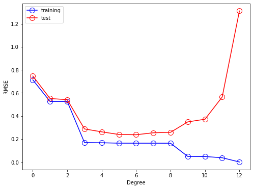
As shown in the next graph, the RMSE of the training data decreases while the RMSE of the testing data increases if the complexity of the model (i.e., degree of polynomial functions) increases.

np.random.seed(11223)
x_train, t_train = create_data(sinusoidal, 13, 0.25)

x_test = np.linspace(0, 1, 100)
t_test = sinusoidal(x_test)

polymodels = [np.poly1d(np.polyfit(x_train, t_train, degree)) for degree in range(13)]

training_errors = [np.sqrt(np.mean((t_train - polymodel(x_train)) ** 2)) for polymodel in polymodels]
test_errors = [np.sqrt(np.mean((t_test + np.random.normal(scale=0.25, size=len(x_test)) - polymodel(x_test)) ** 2))
               for polymodel in polymodels]

plt.figure(figsize=(8, 6))
plt.plot(training_errors, 'o-', mfc="none", mec="b", ms=10, c="b", label="training")
plt.plot(test_errors, 'o-', mfc="none", mec="r", ms=10, c="r", label="test")
plt.legend()
plt.xlabel("Degree")
plt.ylabel("RMSE")
plt.show()

toggle()

show code

Probability Distributions

Probability theory plays the central role in the solution of learning problems.

Bernoulli Distribution

\begin{align*} \text{Bern}(k|\theta) = \left\{ \begin{aligned} & \theta && \text{if } k = 1 \\ & 1-\theta && \text{if } k = 0 \end{aligned} \right. \end{align*}

Binomial Distribution

\begin{align*} \text{Binom}(k|n,\theta) = \left( \begin{array}{c} n \\ k \end{array} \right) \theta^k (1-\theta)^{n-k} = \frac{n!}{k!(n-k)!} \theta^k (1-\theta)^{n-k} \quad \forall k=0, \ldots, n \end{align*}

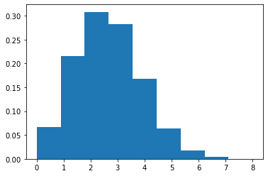
We note \(\text{Bern}(k|\theta) = \text{Binom}(k|1,\theta)\). The plot shows the probability density function (histogram) of binomial distribution with \(n=10\) and \(\theta=0.25\).

data = stats.binom.rvs(10, 0.25, size=10000)
plt.hist(data, bins=data.max()+1, density=True)
plt.show()
toggle()

show code

Beta Distribution

\begin{align*} \text{Beta}(\theta|a,b) = \frac{\Gamma(a+b)}{\Gamma(a)\Gamma(b)} \theta^{a-1} \theta^{b-1} \end{align*}

and

\begin{align*} E(\theta) = \frac{a}{a+b} \end{align*}

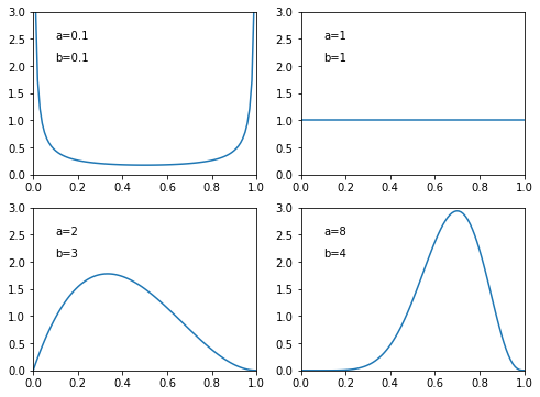
The plots show the probability density function of Beta distribution with different \(a\) and \(b\) values.

x = np.linspace(0, 1, 100)
plt.figure(figsize=(8, 6))
for i, [a, b] in enumerate([[0.1, 0.1], [1, 1], [2, 3], [8, 4]]):
    plt.subplot(2, 2, i + 1)
    beta = stats.beta(a, b)
    plt.xlim(0, 1)
    plt.ylim(0, 3)
    plt.plot(x, beta.pdf(x))
    plt.annotate("a={}".format(a), (0.1, 2.5))
    plt.annotate("b={}".format(b), (0.1, 2.1))
plt.show()

toggle()

show code

Gaussian Distribution

For a \(n\)-dimensional vector \(\mathbf{x}\), the multivariate Gaussian distribution takes the form

\begin{align*} \mathcal{N}(\mathbf{x}|\mu, \Sigma) = \frac{1}{(2 \pi)^{n/2}} \frac{1}{|\Sigma|^{1/2}} \exp \left( -\frac{1}{2} (\mathbf{x} - \mu)^{\intercal} \Sigma^{-1} (\mathbf{x} - \mu) \right) \end{align*}

When \(n=1\), we have the form

\begin{align*} \mathcal{N}(x|\mu, \sigma) = \frac{1}{\sqrt{2 \pi} \sigma} \exp \left( -\frac{1}{2 \sigma^2} (x - \mu)^2 \right) \end{align*}

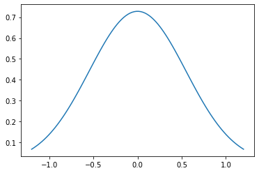
The plot shows the probability density function of Gaussian (normal) distribution.

x = np.linspace(-1.2, 1.2, 100)
plt.plot(x, stats.norm.pdf(x, 0, np.sqrt(0.3)), label="N=0")
plt.show()
toggle()

show code

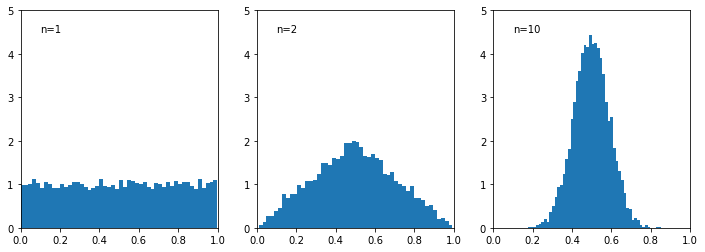
Next, we demonstrate central limit theorem with histogram plots of the mean of \(n\) uniformly distributed numbers

\begin{align*} \frac{x_1 + \ldots + x_n}{n} \end{align*}

for various values of \(n\). We observe that as \(n\) increases, the distribution tends towards a Gaussian.

plt.figure(figsize=(12, 4))

for i, num in enumerate([1, 2, 10]):
    plt.subplot(1, 3, i+1)
    plt.xlim(0, 1)
    plt.ylim(0, 5)
    plt.annotate("n={}".format(num), (0.1, 4.5))
    sample = 0
    for _ in range(num):
        sample = sample + np.random.uniform(0, 1, 10000)
        # np.random.uniform(0, 1, 10000) indicates random 10000 draws of x_{num}
    plt.hist(sample / num, bins=50, density=True)
plt.show()
toggle()

show code

Gamma Distribution

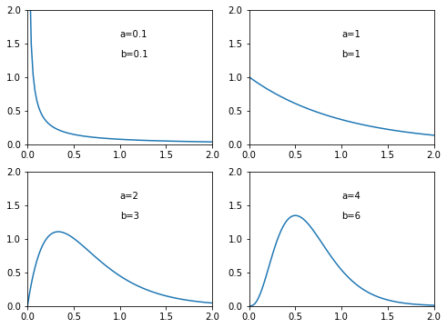
The plots show the probability density function of Gamma distribution.

plt.figure(figsize=(8, 6))

x = np.linspace(0, 2, 100)
for i, [a, b] in enumerate([[0.1, 0.1], [1, 1], [2, 3], [4, 6]]):
    plt.subplot(2, 2, i + 1)
    plt.xlim(0, 2)
    plt.ylim(0, 2)
    plt.plot(x, stats.gamma.pdf(x, a, loc=0, scale=1/b))
    plt.annotate("a={}".format(a), (1, 1.6))
    plt.annotate("b={}".format(b), (1, 1.3))
plt.show()
toggle()

show code

Student’s t Distribution

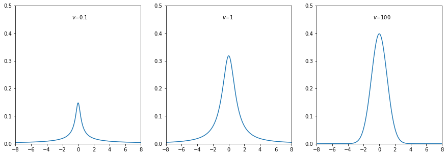
The plots show the probability density function of Student’s t distribution.

plt.figure(figsize=(15, 5))
x = np.linspace(-8, 8, 400)
for i, t in enumerate([0.1, 1, 100]):
    plt.subplot(1, 3, i + 1)
    plt.xlim(-8, 8)
    plt.ylim(0, 0.5)
    plt.plot(x, stats.t.pdf(x, t))
    plt.annotate("$v$={}".format(t), (-.8, 0.45))
plt.show()
toggle()

show code

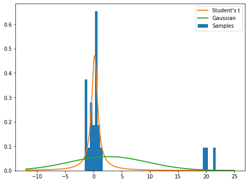
The distribution is used in statistics to estimate the mean of a sample under unknown variance. We fit the data with normal and student’s t distributions. As we can see, the student’s t distribution is more robust because is less sensitive to outliers.

plt.figure(figsize=(8, 6))
X = np.random.normal(size=20)
X = np.concatenate([X, np.random.normal(loc=20., size=3)])
plt.hist(X.ravel(), bins=50, normed=1., label="Samples")

x = np.linspace(-12, 25, 1000)
plt.plot(x, stats.t.pdf(x, *stats.t.fit(X)), label="Student's t", linewidth=2)
plt.plot(x, stats.norm.pdf(x, *stats.norm.fit(X)), label="Gaussian", linewidth=2)
plt.legend()
plt.show()
toggle()

show code

The Frequentist View

Let \(x\) be a random variable and we are trying to estimate its mean \(\theta\). The frequentist believes the true mean \(\theta\) is a fixed value. We have an unbiased estimate after \(n\) observations \(x_1, \ldots, x_n\),

\begin{align*} \theta_n = \frac{1}{n} \sum_{i=1}^{n} x_i \end{align*}

Our estimate of the variance of \(x\) is

\begin{align*} \sigma^2_n = \frac{1}{n-1} \sum_{i=1}^{n} \left( x_i - \theta_n \right)^2 \end{align*}

The estimate of mean and variance of \(x\) can be written recursively as follows

\begin{align*} \theta_n &= \left(1-\frac{1}{n}\right) \theta_{n-1} + \frac{1}{n} x_n \\ \sigma^2_n &= \left\{\begin{aligned} &\frac{1}{n} \left( x_n - \theta_{n-1} \right)^2 && n=2 \\ &\frac{n-2}{n-1} \theta^2_{n-1} + \frac{1}{n} \left( x_n - \theta_{n-1} \right)^2 && n>2 \end{aligned} \right. \end{align*}

The estimate \(\theta_n\) is a random variable because it is computed from other random variables, namely \(x_1, \ldots, x_n\), and random samples. The estimate of the variance of the estimator is

\begin{align*} \bar{\sigma}^2_n = \frac{1}{n} \sigma^2_n \end{align*}

hide_comment()

show comment

Theorem: We have - \(\theta_n\) is an unbiased estimate of \(\theta\)

• \(\sigma^2_n\) is an unbiased estimate of Var(\(x\))

• \(\bar{\sigma}^2_n\) is an unbiased estimate of Var(\(\theta_n\))

Proof: \begin{align*} E(\theta_n) &= \frac{1}{n} \sum_{i=1}^{n} E(x_i) = \theta \\ & \\ E(\sigma^2_{n}) &= \frac{1}{n-1} E \left( \sum_{i=1}^{n} (x_i - \theta_{n})^2\right) \\ &= \frac{1}{n-1} E \left( \sum_{i=1}^{n} x^2_i - 2\sum_{i=1}^{n} x_i \theta_{n} + \sum_{i=1}^{n} \theta^2_{n} \right) \\ &= \frac{1}{n-1} \left( \sum_{i=1}^{n} E \left( x^2_i \right) - 2 E \left( \theta_{n} \sum_{i=1}^{n} x_i \right) + E\left(\sum_{i=1}^{n} \theta^2_{n} \right) \right) \\ &= \frac{1}{n-1} \left( \sum_{i=1}^{n} E \left( x^2_i \right) - 2 n E \left( \theta_{n} \frac{1}{n}\sum_{i=1}^{n} x_i \right) + n E\left(\theta^2_{n} \right) \right) \\ &= \frac{1}{n-1} \left( \sum_{i=1}^{n} E \left( x^2_i \right) - 2 n E \left( \theta^2_{n} \right) + n E\left(\theta^2_{n} \right) \right) \\ &= \frac{1}{n-1} \left( \sum_{i=1}^{n} E \left( x^2_i \right) - n E \left( \theta^2_{n} \right) \right) \\ &= \frac{1}{n-1} \left( \sum_{i=1}^{n} (\sigma^2 + \mu^2) - n \left( \text{Var} \left( \theta_{n} \right) + E^2(\theta_{n}) \right) \right)\\ &= \frac{n}{n-1} \left(\sigma^2 - \text{Var} \left( \theta^2_{n} \right) \right) \\ &= \frac{n}{n-1} \left(\sigma^2 - \text{Var} \left( \frac{1}{n} \sum_{i=1}^{n} x_i \right)\right) \\ &= \frac{n}{n-1} \left(\sigma^2 - \frac{1}{n^2} \sum_{i=1}^{n} \text{Var} \left( x_i \right) \right)\\ &= \frac{n}{n-1} \left(\sigma^2 - \frac{1}{n^2} \sum_{i=1}^{n} \sigma^2 \right) = \sigma^2 \\ & \\ \text{Var}(\theta_n) &= \text{Var}\left(\frac{1}{n} \sum_{i=1}^n x_i\right) \\ & = \frac{1}{n^2} \text{Var}\left(\sum_{i=1}^n x_i\right) \\ & = \frac{1}{n^2} n \text{Var}\left(\mathbf{x}\right) \quad \text{because of i.i.d. observations} \\ & = \frac{1}{n} \sigma^2_n \end{align*}

\(\blacksquare\)

The Bayesian View

Again, we try to estimate the mean \(\theta\) of a random variable \(x\). The Bayesian perspective considers \(\theta\) as a random variable. In other words, any number whose value we do not know is interpreted as a random variable, and the distribution of this random variable represents our belief about how likely \(\theta\), is to take on certain values.

Bayes’ theorem takes the form

\begin{align*} p(\theta|\mathcal{D}) = \frac{p(\mathcal{D}|\theta) p(\theta)}{p(\mathcal{D})}, \end{align*}

where \(\mathcal{D} = \{x_1, x_2, \ldots, x_n\}\) is the observed dataset, and

• \(p(\theta)\) is a prior probability distribution which captures our assumptions about about \(\theta\) before observing the data;

• \(p(\mathcal{D}|\theta)\) is called the likelihood function and expresses how probable the observed data set is for different settings of the parameter vector \(\theta\) through the conditional probability;

• \(p(\mathcal{D})\) plays as a normalization constant constant because it does not depend on \(\theta\). It ensures that the posterior distribution on the left-hand side is a valid probability density and integrates to one.

Conjugacy: Bayes rule can be simply expressed as

\begin{align*} \text{posterior} \propto \text{likelihood} \times \text{prior} \end{align*}

We would prefer to choose a prior such that the posterior distribution have the same functional form as the prior. This property is called conjugacy, and the prior is called conjugate prior. We will see several examples later.

If the posterior distribution have the same functional form as the prior, then the Bayes rule can be easily applied recursively.

Learning with Gaussian Prior

Consider a single Gaussian random variable \(x\) with known variance \(\sigma^2\). Our task is to infer the mean \(\theta\) given a set of \(n\) observations \(\{x_1, \ldots, x_n\}\). Assume the prior distribution is Gaussian \(p(\theta) = \mathcal{N} (\theta | \mu_0, \sigma^2_0)\).

After \(n\) observations, we have learned that \(\theta\) follows \(\mathcal{N} (\theta | \mu_n, \sigma^2_n)\) where

\begin{align*} \frac{1}{\sigma_n^2} &= \frac{n}{\sigma^2} + \frac{1}{\sigma_0^2} \\ \mu_n &= \left( \frac{n}{\sigma^2} + \frac{1}{\sigma_0^2} \right)^{-1} \left( \frac{\mu_0}{\sigma^2_0} + \frac{1}{\sigma^2} \sum_{i=1}^{n} x_i \right). \end{align*}

It gives the updating equation \begin{align*} \frac{1}{\sigma_n^2} &= \frac{1}{\sigma^2_{n-1}} + \frac{1}{\sigma_0^2} \\ \mu_n &= \sigma_n^2 \left( \frac{\mu_{n-1}}{\sigma^2_{n-1}} + \frac{1}{\sigma^2} x_n \right), \end{align*}

as our learning procedure.

hide_comment()

show comment

Proof:

The likelihood function is

\begin{align*} p(\{x_1, \ldots, x_n\} | \theta) = \prod_{i=1}^{n} p(x_n | \theta) = \frac{1}{(2\pi \sigma^2)^{n/2}} \exp \left\{ -\frac{1}{2 \sigma^2} \sum_{i=1}^{n} (x_n - \theta)^2\right\} \end{align*}

The posterior distribution is given by

\begin{align*} p(\theta|\{x_1, \ldots, x_n\}) \propto p(\{x_1, \ldots, x_n\} | \theta) p(\theta) \end{align*}

where \(p(\theta) = \mathcal{N} (\theta | \mu_0, \sigma^2_0)\) is our prior. It gives

\begin{align*} p(\theta|\{x_1, \ldots, x_n\}) \propto \frac{1}{(2\pi \sigma^2)^{n/2}} \exp \left\{ -\frac{1}{2 \sigma^2} \sum_{i=1}^{n} (x_i - \theta)^2\right\} \frac{1}{(2\pi \sigma^2_0)^{1/2}} \exp \left\{ -\frac{(\theta - \mu_0)^2}{2 \sigma^2_0}\right\} \end{align*}

The exponent takes the form

\begin{align} -\frac{1}{2 \sigma^2} \sum_{i=1}^{n} (x_n - \theta)^2 -\frac{(\theta - \mu_0)^2}{2 \sigma^2_0} = -\frac{\theta^2}{2} \left( \frac{1}{\sigma^2_0} + \frac{n}{\sigma^2} \right) + \theta \left( \frac{\mu_0}{\sigma^2_0} + \frac{1}{\sigma^2} \sum_{i=1}^{n} x_i \right) \label{eqn_norm_1} \end{align}

Because of conjugacy, we have

\begin{align*} p(\theta|\{x_1, \ldots, x_n\}) = \mathcal{N}(\mu_n, \sigma_n^2) \end{align*}

and the exponent of \(\mathcal{N}(\mu_n, \sigma_n^2)\) takes the form

\begin{align} -\frac{1}{2\sigma^2_n} (\theta - \mu_n)^2 = -\frac{\theta^2}{2 \sigma^2_n} + \frac{\theta \mu_n}{\sigma^2_n} + \text{constant} \label{eqn_norm_2} \end{align}

Since both \eqref{eqn_norm_1} and \eqref{eqn_norm_2} represent the posterior distribution. They should have the same coefficient for terms \(\theta^2\) and \(\theta\), respectively. Thus, we have

\begin{align*} \frac{1}{\sigma_n^2} &= \frac{n}{\sigma^2} + \frac{1}{\sigma_0^2} \\ \frac{\mu_n}{\sigma^2_n} &= \frac{\mu_0}{\sigma^2_0} + \frac{1}{\sigma^2} \sum_{i=1}^{n} x_i. \end{align*}

\(\blacksquare\)

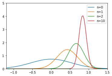
The code shows the learning process.

• The prior distribution is gaussian(0, 0.3)

• The data set is generated from gaussian(0.8, 0.1)

• After observing data sequentially, we can eventually learn the ‘true’ distribution gaussian(0.8, 0.1)

class gaussian:
    def __init__(self, mu, var):
        self.parameter = {}
        self.mu = mu
        self.var = var
        self.tau = 1/var

    @property
    def var(self):
        return self.parameter["var"]

    @property
    def tau(self):
        return self.parameter["tau"]

    @var.setter
    def var(self, var):
        self.parameter["var"] = var
        self.parameter["tau"] = 1 / var

    @tau.setter
    def tau(self, tau):
        self.parameter["tau"] = tau
        self.parameter["var"] = 1 / tau

mu = gaussian(0, 0.3)
data = gaussian(0.8, 0.1)

x = np.linspace(-1.2, 1.5, 100)
plt.plot(x, stats.norm.pdf(x, mu.mu, np.sqrt(mu.var)), label="n=0")

x_train = np.random.normal(loc=data.mu, scale=np.sqrt(data.var), size=10)

for beg, end in [[0,1],[1,2],[2,10]]:
    seq_x = x_train[beg:end]
    n = len(seq_x)
    mu_ml = np.mean(seq_x, 0)
    mu.mu = (data.var * mu.mu +  n * mu.var * mu_ml) / (data.var + n * mu.var)
    mu.tau = mu.tau + n * data.tau
    plt.plot(x, stats.norm.pdf(x, mu.mu, np.sqrt(mu.var)), label="n={}".format(end))

plt.xlim(-1.2, 1.5)
plt.ylim(0, 5)
plt.legend()
plt.show()
toggle()

show code

Learning Correlated Gaussian Prior

A particularly important problem class in learning involves correlated multiple choices. Correlated beliefs are a particularly powerful device in learning, allowing us to generalize the results of a single observation to other alternatives that we have not directly measured.

Consider a multivariate Gaussian random variable \(\mathbf{x}\) with known covariance matrix \(\Sigma\). Our task is to infer the mean vector \(\theta\) given a single observation on the \(i\)th component \(x_i\) with known variance \(\sigma^2_i\).

For example, a physician is trying to treat diabetes using a treatment of three drugs, where she observes the drop in blood sugar from a course of a particular treatment. If one treatment produces a better-than-expected response, this would also increase our belief of the response from other treatments that have one or two drugs in common.

Suppose the prior is \(p(\theta) = \mathcal{N}(\mu_{0}, \Sigma_{0})\). Then, the posterior distribution \(p(\theta|x_i) = \mathcal{N}(\mu_{(1)}, \Sigma_{(1)})\) with updating equations

\begin{align*} \Sigma^{-1}_{(1)} & = \Sigma^{-1}_0 + \frac{1}{\sigma^2_i} e_i e_i^\intercal \\ \mu_{(1)} & = \Sigma_{(1)} \left( \Sigma^{-1}_0 \mu_0 + \frac{1}{\sigma^2_i} x_i e_i \right) \end{align*}

where the subscript (1) indicating the first step learning and \(e_i\) is the unit vector.

hide_comment()

show comment

Proof of the updating equations:

The posterior \(p(\theta|x_i)\) is

\begin{align*} p(\theta|x_i) \propto p(x_i|\theta) p(\theta) \end{align*}

The exponent of the posterior \(p(\theta|x_i)\) is

\begin{align*} &-\frac{1}{2 \sigma^2_i} (x_i - \theta_i)^2 -\frac{1}{2} (\theta-\mu_0)^\intercal \Sigma^{-1}_0 (\theta-\mu_0) \\ =&-\frac{1}{2} \theta ^\intercal \Sigma^{-1} \theta -\frac{\theta^2_i}{2 \sigma^2_i} + \theta^\intercal \Sigma^{-1}_0 \mu_0 + \frac{1}{ \sigma^2_i} x_i \theta_i + \text{constant} \\ =&-\frac{1}{2} \theta ^\intercal \Sigma^{-1}_0 \theta -\frac{1}{2\sigma^2_i} \theta^\intercal e_i e_i^\intercal \theta + \theta^\intercal \Sigma^{-1}_0 \mu_0 + \frac{1}{ \sigma^2_i} x_i \theta^\intercal e_i + \text{constant} \\ =&-\frac{1}{2} \theta ^\intercal \left( \Sigma^{-1}_0 + e_i e_i^\intercal\right) \theta + \theta^\intercal \left( \Sigma^{-1}_0 \mu_0 + \frac{1}{ \sigma^2_i} x_i e_i \right) + \text{constant}. \end{align*}

Therefore, we have updating equation \begin{align*} \Sigma^{-1}_{(1)} & = \Sigma^{-1}_0 + \frac{1}{\sigma^2_i} e_i e_i^\intercal \\ \mu_{(1)} & = \Sigma_{(1)} \left( \Sigma^{-1}_0 \mu_0 + \frac{1}{\sigma^2_i} x_i e_i \right) \end{align*}

where the subscript (1) indicating the first step learning. Note that Sherman-Morrison formula,

\begin{align*} (A + u u^\intercal)^{-1} = A^{-1} - \frac{A^{-1} u u^\intercal A^{-1}}{1 + u^{\intercal} A^{-1} u} \end{align*}

with invertible \(A\), can be applied to simplify the inverse calculation for \(\Sigma^{-1}_{(1)}\).

\(\blacksquare\)

Example:

Suppose we have mean and covariance \begin{align*} \mu_0 = \left( \begin{array}{l} 20 \\ 16 \\ 22 \end{array} \right) \text{ and } \Sigma_0 = \left( \begin{array}{lll} 12 & 6 & 3 \\ 6 & 7 & 4 \\ 3 & 4 & 15 \end{array} \right) \end{align*}

of the prior and the variance of \(x_3\) is 9. After we observe a value of 19 for \(x_3\), our beliefs are updated as follows:

from numpy.linalg import inv

mu = np.array([20, 16, 22])
sigma = np.array([[12, 6, 3], [6, 7, 4], [3, 4, 15]])

e = np.zeros(3)
e[-1] = 1

observed = 19
var = 9

updated_sigma = inv(np.outer(e, e)/var + inv(sigma))

updated_mu = updated_sigma.dot(inv(sigma).dot(mu) + 1/var * observed * e)
print("updated mu = \n",updated_mu)
print("updated sigma = \n",updated_sigma)
toggle()

updated mu =
 [19.625 15.5   20.125]
updated sigma =
 [[11.625       5.5         1.125     ]
 [ 5.5         6.33333333  1.5       ]
 [ 1.125       1.5         5.625     ]]

show code

Learning Probabilities

Our objective is to learn the probability that a certain event will occur.

• For example, in a medical setting, our observations might simply be whether or not a certain medical treatment is successful. Such an observation can be modeled as a Bernoulli random variable, which is equal to 1 (success) with probability \(\theta\), and 0 (failure) with probability \(1 - \theta\). The success probability \(\theta\) is the unknown true value in this case.

• For example, instead of merely measuring the success or failure of a medical treatment, we also consider cases where the treatment is generally effective, but causes certain side effects. Each observation can be classified as belonging to one of \(K > 2\) different categories.

The beta-Bernoulli Model

To estimate \(\theta\), the likelihood function \(\text{Bern}(k|\theta)\) takes the form of the product of factors of the form \(\theta^k(1-\theta)^{1-k}\) where \(k \in \{0,1\}\) is the binary observation. If we choose a prior to be proportional to powers of \(\theta\) and \((1-\theta)\), then the posterior distribution, which is proportional to the product of the prior and the likelihood function, will have the same functional form as the prior.

Let the prior be \(\text{Beta}(\theta | a, b)\) with

\begin{align*} \text{Beta}(\theta | a, b) = \frac{\Gamma(a+b)}{\Gamma(a)+\Gamma(b)} \theta^{a-1} (1-\theta)^{b-1} \end{align*}

Recall that it has mean \(a/(a+b)\) and variance \(ab/((a+b)^2+(a+b+1))\).

Because

\begin{align*} \text{Bern}(k|\theta) \times \text{Beta}(\theta | a, b) & \propto \theta^k(1-\theta)^{1-k} \times \theta^{a-1}(1-\theta)^{b-1} \propto \theta^{(a+k)-1}(1-\theta)^{(b+(1-k))-1} \\ & \propto \text{Beta}(\theta | a+k, b+1-k) \end{align*}

The posterior distribution of \(\theta\) is

\begin{align*} \underbrace{\text{Beta}(\theta | a+k, b+1-k)}_{posterior} \propto \underbrace{\text{Bern}(k|\theta)}_{likelihood} \times \underbrace{\text{Beta}(\theta | a, b)}_{prior} \end{align*}

For a single observation of the success (with \(k=1\)) or failure (with \(k=0\)), the equation shows

\begin{align*} E(\theta) &= \frac{a+k}{(a+k)+(b+1-k)} = \frac{a+k}{a+b+1} \end{align*}

our updated estimate of the probability \(\theta\).

It is easy to note that, after observing a data set of \(m\) successes and \(l\) failures, the posterior distribution of \(\theta\) is \(\text{Beta}(\theta | m+a, l+b)\). So,

\begin{align*} E(\theta) &= \frac{m+a}{m+a+l+b} \\ \text{Var}(\theta) &= \frac{(m+a)(l+b)}{(m+a+l+b)^2+(m+a+l+b+1)} \end{align*}

Example: We demonstrate the learning process after a success (a single observation with \(k=1\)):

\begin{align*} \underbrace{\text{Beta}(\theta | a+1, b)}_{posterior} \propto \underbrace{\text{Bern}(k = 1|\theta)}_{likelihood} \times \underbrace{\text{Beta}(\theta | a, b)}_{prior}. \end{align*}

where

• prior: a beta distribution

• likelihood: a binary random variable given \(\theta\)

• posterior: only the values with a single observation of \(k=1\) are kept as posterior

The code works as follows.

1. We derive a set of \(\theta\) values following prior distribution

2. Since the observation is \(k=1\), a Bernoulli distribution with parameter \(\theta\) generating a value \(1\) indicates that \(\theta\) is “reasonable” and consistent with the observation.

3. We keep all “reasonable” \(\theta\) as posterior. Posterior is what we have learned from the observation based on prior.

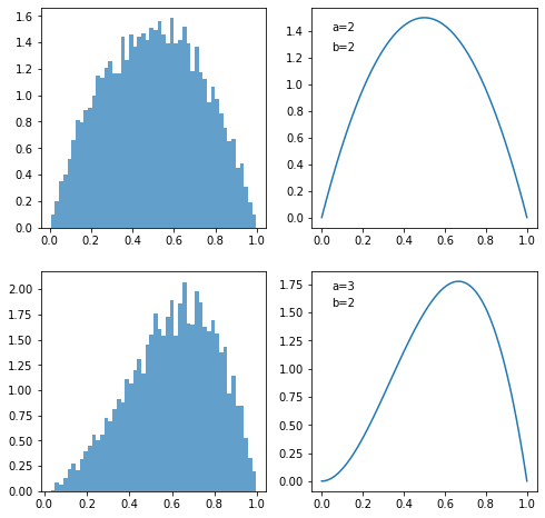
Two plots on the left are based on simulation and two plots on the right are based on theoretical beta distribution. As shown in the plots, the learning process indeed induces beta posterior distribution.

x = np.linspace(0, 1, 100)

# generate 10,000 mu values from the prior distribution
prior = stats.beta.rvs(2, 2, size=10000)

# the likelihood follows bernoulli distribution with a given mu
likelihood = stats.bernoulli.rvs(prior, size=prior.shape)

posterior = (likelihood*prior)[(likelihood*prior)!=0]

fig, axes = plt.subplots(2, 2, figsize=(8,8))
axes[0,0].hist(prior, density=True, histtype='stepfilled', alpha=0.7, bins=50)
axes[0,1].plot(x, (stats.beta(2,2)).pdf(x))
axes[0,1].annotate("a={}".format(2), (0.05, 1.4))
axes[0,1].annotate("b={}".format(2), (0.05, 1.25))

axes[1,0].hist(posterior, density=True, histtype='stepfilled', alpha=0.7, bins=50)
axes[1,1].plot(x, (stats.beta(3,2)).pdf(x))
axes[1,1].annotate("a={}".format(3), (0.05, 1.7))
axes[1,1].annotate("b={}".format(2), (0.05, 1.55))
plt.show()
np.round(stats.beta.fit(posterior, floc=0, fscale=1)[:2],3)
print("Based on simulation, posterior beta distribution has [a,b]={}"\
      .format(np.round(stats.beta.fit(posterior, floc=0, fscale=1)[:2],3)))
toggle()

Based on simulation, posterior beta distribution has [a,b]=[2.991 1.973]

show code

The multivariate-Dirichlet Model

Our goal is to learn the probabilities of \(K\) alternatives \(\theta = (\theta_1, \ldots, \theta_K)\), where the probability \(\theta_k\) for the \(k\)th alternative, base on \(n\) observations \(\mathbf{x}^1, \ldots, \mathbf{x}^n\). The observations are represented in 1-of-\(K\) scheme that

\begin{align*} \mathbf{x}^i = (0, \ldots, 0, \underbrace{1}_{k \text{th}}, 0, \ldots, 0)_{1 \times K} \end{align*}

indicates the \(i\)th observation is the \(k\)th alternative. Therefore, the distribution of an observation \(x\) is given

\begin{align*} p(\mathbf{x}|\theta) = \prod_{k=1}^{K} \theta_k^{x_k} \end{align*}

Then, the likelihood function takes the form

\begin{align*} p(\mathbf{x}^1, \ldots, \mathbf{x}^n|\theta) = \prod_{i=1}^{n} \prod_{k=1}^{K} \theta_k^{\mathbf{x}^i_k} = \prod_{k=1}^{K} \theta_k^{\sum_{i=1}^n x^i_k} \end{align*}

The conjugate prior is given by Dirichlet distribution

\begin{align*} \text{Dir}(\theta| \alpha^{(0)}_0,\ldots,\alpha^{(0)}_K) = \frac{\Gamma(\alpha^{(0)}_0)}{\Gamma(\alpha^{(0)}_1) \cdots \Gamma(\alpha^{(0)}_K)} \prod_{k=1}^{K} \theta^{\alpha^{(0)}_k-1}_k \end{align*}

with \(\alpha^{(0)}_0 = \sum_{i=1}^{K} \alpha^{(0)}_i\). The posterior distribution is in the form

\begin{align*} p(\mathbf{x}^1, \ldots, \mathbf{x}^n|\theta) \text{Dir}(\theta| \alpha^{(0)}_0,\ldots,\alpha^{(0)}_K) & \propto \text{Dir}\left(\theta| \alpha^{(0)}_0+n,\alpha^{(0)}_1+\sum_{i=1}^n \mathbf{x}^i_1, \ldots,\alpha^{(0)}_K+\sum_{i=1}^n \mathbf{x}^i_K\right) \\ & \equiv \text{Dir}\left(\theta| \alpha^{(n)}_0,\alpha^{(n)}_1, \ldots,\alpha^{(n)}_K \right) \end{align*}

Our estimate of the probability of observing an outcome in category \(k\) given

\begin{align*} \theta^{(n)}_k = \frac{\alpha^{(n)}_k}{\alpha^{(n)}_1 + \cdots + \alpha^{(n)}_K} = \frac{\alpha_k+\sum_{i=1}^n \mathbf{x}^i_k}{\alpha_0+n} \end{align*}

Our belief is updated as follows

\begin{align*} \alpha^{(n)}_k = \left\{ \begin{aligned} &\alpha^{(n-1)}_k + 1 && \text{if observation belongs to category } k,\\ &\alpha^{(n-1)}_k && \text{otherwise.} \end{aligned} \right. \end{align*}

Bayes’ Estimate

Consider a biased coin. Let \(\theta\) be the probability of showing head, i.e., \(p(x=1|\theta) = \theta\), for a biased coin. If one toss comes up head, we can estimate \(\theta\) with

Maximum Likelihood Estimation (MLE)

\begin{align*} \hat{\theta} = \text{argmax}_{\theta} ~ p(x=1|\theta) = \text{argmax}_{\theta} ~ \theta = 1 \end{align*}

We simply maximize likelihood function (no need to use log).

Maximum A Posteriori (MAP)

Suppose the prior \(p(\theta) = 1\) is uniform distribution on \([0,1]\)

\begin{align*} p(\theta|x=1) &= \frac{p(x=1|\theta)p(\theta)}{p(x=1)} = \frac{p(x=1|\theta)}{p(x=1)} \\ \Rightarrow \hat{\theta} &= \text{argmax}_{\theta} ~ p(\theta|x=1) = \text{argmax}_{\theta} ~ p(x=1|\theta) = \text{argmax}_{\theta} ~ \theta = 1 \end{align*}

We note that uniform prior cannot solve over-fitting.

Now, suppose the prior \(p(\theta) = \text{Beta}(\theta|a,b)\). Because of conjugacy, the posterior \(p(\theta|x=1) = \text{Beta}(\theta|a+1,b)\).

\begin{align*} \hat{\theta} = \text{argmax}_{\theta} ~ p(\theta|x=1) = \text{argmax}_{\theta} \theta^a (1-\theta)^{b-1} = \frac{a}{a+b-1} \end{align*}

Bayes’ Estimate

Suppose \(p(\theta) = 1\) is uniform distribution on \([0,1]\). Note that

\begin{align*} p(x=1) = \int_{0}^{1} p(x=1|\theta)p(\theta) d\theta = \int_{0}^{1} \theta d\theta = \frac{1}{2} \end{align*}

The posterior distribution is \begin{align*} p(\theta|x=1) &= \frac{p(x=1|\theta)p(\theta)}{p(x=1)} = \frac{p(x=1|\theta)}{p(x=1)} = 2 \theta \\ \hat{\theta} &= E(\theta|x=1) = \int_0^1 \theta p(\theta|x=1) d\theta = \int_0^1 2\theta^2 d\theta = \frac{2}{3} \end{align*}

Summary

In summary, there are three approaches to estimate parameter \(\theta\) with independent observations \(\mathcal{D}\):

Maximum Likelihood (ML):

We find the largest value to the likelihood

\begin{align*} \hat{\theta}_{\text{ML}} = \text{argmax}_{\theta} ~p(\mathcal{D}|\theta) = \prod_{i=1}^{n} p(\mathbf{x}_i|\theta) \end{align*}

Maximum A Posteriori (MAP):

We find the largest value to the posterior

\begin{align*} \hat{\theta}_{\text{MAP}} = \text{argmax}_{\theta} ~p(\theta|\mathcal{D}) = \text{argmax}_{\theta} \frac{p(\mathcal{D}|\theta) p(\theta)}{p(\mathcal{D})} = \text{argmax}_{\theta} ~ p(\mathcal{D}|\theta) p(\theta) \end{align*}

Bayesian:

We first calculates the posterior distribution \(p(\theta|\mathcal{D})\) fully where

\begin{align*} p(\theta|\mathcal{D}) = \frac{p(\mathcal{D}|\theta) p(\theta)}{p(\mathcal{D})}. \end{align*}

Then the estimate \(\hat{\theta}\) can be obtained by the mean, \(\textrm{E}_{\theta}(p(\theta|\mathcal{D}))\), or mode of the distribution.

Both ML and MAP return only single and specific values for the parameter \(\theta\).

• MAP estimation “pulls” the estimate toward the prior.

• The more focused:nbsphinx-math:footnote{centered around mean with low variance} our prior belief, the larger the pull toward the prior.

• The prior may have parameters \(p(\theta; \alpha)\) plays a “smoothing role”. For example, \(\alpha\) is hyperparameter that can be found by evidence approximate.

Bayesian estimation, by contrast, calculates fully the posterior distribution \(p(\theta|\mathcal{D})\). Note that the probability of evidence \(p(\mathcal{D})\) is a constant where

\begin{align*} p(\mathcal{D}) = \int p(\mathcal{D}|\theta) p(\theta) d\theta. \end{align*}

\(p(\mathcal{D})\) is ignored in MAP but is considered in Bayes. \(\theta\) can have many possible estimate values following the estimated posterior distribution. For example,

• We may choose \(\textrm{E}(\theta)\) assuming \(\textrm{Var}(\theta)\) is small.

• We may declare no good estimate if \(\textrm{Var}(\theta)\) is too large, since \(\textrm{Var}(\theta)\) expresses confidence.

MLE for the Gaussian

Suppose that a data set of observations \(\mathbf{x} = (x_1, . . . , x_n)^\intercal\), representing \(n\) observations of the scalar variable \(x\), are drawn independently from a Gaussian distribution whose mean \(\mu\) and variance \(\sigma^2\) are unknown, and we would like to determine these parameters from the data set.

Because the data set \(\mathbf{x}\) is i.i.d., the probability

\begin{align*} p(\mathbf{x}|\mu, \sigma^2) = \prod_{i=1}^{n} \mathcal{N} (x_i|\mu, \sigma^2) \end{align*}

gives the likelihood function and

\begin{align} \ln p(\mathbf{x}|\mu, \sigma^2) = -\frac{1}{2\sigma^2} \sum_{i=1}^{n} (x_i - \mu)^2 - \frac{n}{2} \ln \sigma^2 - \frac{n}{2} \ln(2 \pi) \label{eqn_normal_ml} \end{align}

Maximizing \eqref{eqn_normal_ml} with respect to \(\mu\), we obtain the maximum likelihood solution

\begin{align*} \mu_{ML} = \frac{1}{n} \sum_{i=1}^{n} x_i \end{align*}

which is the sample mean. Maximizing \eqref{eqn_normal_ml} with respect to \(\sigma^2\), we obtain

\begin{align*} \sigma^2_{ML} = \frac{1}{n} \sum_{i=1}^{n} (x_i - \mu_{ML})^2 \end{align*}

which is the sample variance measured with respect to the sample mean. Note that \(\sigma^2_{ML}\) is a biased estimate of the true variance \(\sigma^2\).

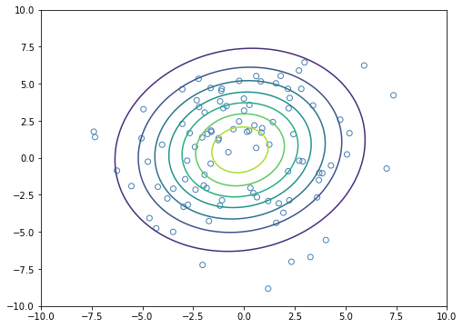
The plot shows the maximum likelihood estimation for the Gaussian.

x_train = stats.norm.rvs(scale=3., size=(100, 2))

mu_ml = np.mean(x_train, axis=0)
cov_ml = np.atleast_2d(np.cov(x_train.T, bias=True))

plt.figure(figsize=(8, 6))
x, y = np.meshgrid(np.linspace(-10, 10, 100), np.linspace(-10, 10, 100))
p = stats.multivariate_normal.pdf(np.array([x, y]).reshape(2, -1).T, mean=mu_ml, cov=cov_ml).reshape(100, 100)
plt.scatter(x_train[:, 0], x_train[:, 1], facecolor="none", edgecolor="steelblue")
plt.contour(x, y, p)
plt.show()
toggle()

show code

Mixtures of Gaussians

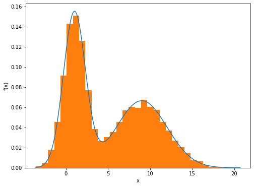
We see that the data set forms two dominant clumps, and that a simple Gaussian distribution is unable to capture this structure, whereas a linear superposition of two Gaussians gives a better characterization of the data set.

By using a sufficient number of Gaussians, and by adjusting their means and covariances as well as the coefficients in the linear combination, almost any continuous density can be approximated to arbitrary accuracy.

We therefore consider a superposition of \(K\) Gaussian densities of the form

\begin{align*} p(\mathbf{x}) = \sum_{k=1}^{K} \pi_k \mathcal{N} (\mathbf{x} | \mu_k, \Sigma_k) \end{align*}

where

\begin{align*} \sum_{k=1}^{K} \pi_k = 1 \text{ and } 0 \le \pi_k \le 1 \end{align*}

Due to the summation \(\sum_{k=1}^{K}\), the maximum likelihood solution for the parameters

\begin{align*} \ln p(\mathbf{x_1}, \ldots, \mathbf{x_n}| \pi, \mu, \Sigma) = \sum_{i=1}^{n} \ln \left\{ \sum_{k=1}^{K} \pi_k \mathcal{N} (\mathbf{x}_i | \mu_k, \Sigma_k) \right\} \end{align*}

no longer has a closed-form analytical solution.

n = 10000
np.random.seed(12345)
# Parameters of the mixture components
norm_params = np.array([[1, 1.3],
                        [9, 3]])
n_components = norm_params.shape[0]
# Weight of each component, in this case all of them are 1/2
weights = np.ones(n_components, dtype=np.float64) / 2.0
# A stream of indices from which to choose the component
mixture_idx = np.random.choice(len(weights), size=n, replace=True, p=weights)
# y is the mixture sample
y = np.fromiter((stats.norm.rvs(*(norm_params[i])) for i in mixture_idx),
                   dtype=np.float64)

# Theoretical PDF plotting -- generate the x and y plotting positions
xs = np.linspace(y.min(), y.max(), 200)
ys = np.zeros_like(xs)

for (l, s), w in zip(norm_params, weights):
    ys += stats.norm.pdf(xs, loc=l, scale=s) * w

plt.figure(figsize=(8, 6))
plt.plot(xs, ys)
plt.hist(y, normed=True, bins="fd")
plt.xlabel("x")
plt.ylabel("f(x)")
plt.show()
toggle()

show code

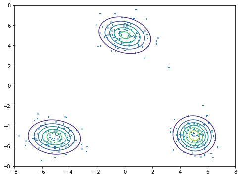
The plot fits data into mixtures of 3 Gaussians by using sklearn package.

from sklearn import mixture

x1 = np.random.normal(size=(100, 2))
x1 += np.array([-5, -5])
x2 = np.random.normal(size=(100, 2))
x2 += np.array([5, -5])
x3 = np.random.normal(size=(100, 2))
x3 += np.array([0, 5])
X = np.vstack((x1, x2, x3))

x_test, y_test = np.meshgrid(np.linspace(-10, 10, 100), np.linspace(-10, 10, 100))
X_test = np.array([x_test, y_test]).reshape(2, -1).T

plt.figure(figsize=(8, 6))
plt.scatter(X[:, 0], X[:, 1], s=3)
Z = np.exp(mixture.GaussianMixture(n_components=3, covariance_type='full').fit(X).score_samples(X_test)).reshape(-1, 100)
plt.contour(x_test, y_test, Z)
plt.xlim(-8, 8)
plt.ylim(-8, 8)
plt.show()
toggle()

show code

The Curse of Dimensionality

Consider inputs uniformly distributed in a p-dimensional unit hypercube. We perform the nearest-neighbor procedure to estimate \(f(x_0) = \text{Avg}_{x_i \in V} x_i\), where \(V\) is a hypercubical neighborhood about the target point \(x_0\) and captures a fraction \(r\) of the observations.

The expected edge length of \(V\) is \(r^{1/p}\), since it includes a fraction \(r\) of the unit volume. Note that, In ten dimensions, to capture 1% or 10% of the data to form a local average, we must cover 63%(\(=0.01^{0.1}\)) or 80%(\(=0.1^{0.1}\)) of the range of each input variable.

Apparently, those neighborhoods are no longer “local”. Also, we cannot reduce \(r\) dramatically as since the fewer observations we average, the higher is the variance of our fit.

Consider \(n\) data points uniformly distributed in a \(p\)-dimensional unit ball centered at \(x_0\), and we consider a nearest-neighbor estimate on \(x_0\). The median distance from \(x_0\) to the closest data point is

\begin{align*} d = \left(1 - \frac{1}{2}^{1/n} \right)^{1/p}. \end{align*}

Let \(V_p(r)\) be the volume of a \(p\)-dimensional ball of radius \(r\). Another manifestation of the curse is that

\begin{align*} \frac{V_p(1)-V_p(1-\epsilon)}{V_p(1)} = 1 - (1-\epsilon)^p \end{align*}

For large \(p\), the value tends to 1 even for small values of \(\epsilon\). Thus, in spaces of high dimensionality, most of the volume of a sphere is concentrated in a thin shell near the surface.

The results indicate that all sample points are close to an edge of the sample for the sparse sampling in high dimensions. The reason that this presents a problem is that prediction is much more difficult near the edges of the training sample. One must extrapolate from neighboring sample points rather than interpolate between them.

hide_comment()

show comment

Show the median distance formula

The volume of a ball of radius \(r\) in \(\Re^p\) is \(\omega_p r^p\), where \(\omega_p\) is a constant depending only on \(p\). The probability that a point, taken uniformly in the unit ball, is within distance \(r\) of the origin is the volume of that ball divided by the volume of the unit ball. So the CDF is

\begin{align*} F(r) = r^p, \; \; \; 0 \leq r \leq 1. \end{align*}

The PDF of the smallest order statistic (the minimum) \(y\) of \(n\) points is

\begin{align*} g(y) = n \left( 1 - F(y) \right)^{n-1} f(y) = n \left( 1 - y^p \right)^{n-1} p y^{p-1} \end{align*}

and its CDF is

\begin{align*} G(y) = 1 - \left( 1 - y^p \right)^{n} \end{align*}

The median \(d\) satisfies \(G(d) = 1/2\).

\(\blacksquare\)

Information Theory

Informtaion can be considered as assigning probablities on a set of different events. Hence, the measure of information content depends on a distribution, says \(q(x)\). A knowledge “a pill normally takes effect after 3 hours” provides following information content

1. the time that a pill takes effect for different people follows a certain distribution;

2. the mean of such a distribution is 3 hours.

Generally speaking, we expect that a machine learning algorithm returns a distribution \(p(x)\) which is “close” to \(q(x)\). The question is how to measure the closeness of two distributions.

Entropy

Given a random state variable \(x\), Our measure of information content will therefore depend on the probability distribution \(p(x)\), and we look for a quantity \(h(x)\) that is a function of the probability \(p(x)\) and that expresses the information content.

An important quantity is called the entropy of the random variable \(x\)

\begin{align*} H[x] = - \sum_{x} p(x) \log_2 p(x) \end{align*}

where we sum over all possible state of \(x\). Entropy is a measure of the average amount of information in terms of the number of bits.

For example, a encoding scheme.

letter	Encoding
A	0
B	1
C	01

is short but extremely flawed, as the message “AB” and the message “C” are indistinguishable (both would be transmitted as 01). In contrast, the encoding scheme

letter	Encoding
A	00001
B	00111
C	11111

is correct, but extremely inefficient because much more bits are necessary to reliably transmit messages.

It is natural to ask what the “best” encoding scheme is. Although the exact answer strongly depends on application, one natural answer is “the correct encoding scheme that minimizes the expected length of a message.” That theoretical minimum is given by the entropy of the message.

For example, suppose a message details the value of a random variable \(X\), defined by

\(x\)	Pr\(\big(X\) \(=\) \(x\big)\)
A	0.5
B	0.25
C	0.125
D	0.125

The entropy of this message is

\begin{align*} H[x] = - \frac{1}{2} \log_2 \frac{1}{2} - \frac{1}{4} \log_2 \frac{1}{4} - \frac{1}{8} \log_2 \frac{1}{8} - \frac{1}{8} \log_2 \frac{1}{8} = 1.75 \text{ bits} \end{align*}

so the expected length of any correct encoding scheme is at least 1.75. In this case, this can be realized with a relatively simple scheme:

letter	Encoding	Length
A	1	1
B	0	2
C	001	3
D	000	3

It can be verified that the above encoding is correct (it is an example of Huffman coding), and it has expected length

\begin{align*} 1 \cdot 0.5 + 2 \cdot 0.25 + 3 \cdot 0.125 + 3 \cdot 0.125 = 1.75, \end{align*}

which is equal to the entropy of the message.

This relation between entropy and shortest coding length is a general one. The noiseless coding theorem (Shannon, 1948) states that the entropy is a lower bound on the number of bits needed to transmit the state of a random variable.

The uniform distribution has a larger entropy than the nonuniform one. Consider a random variable x having 8 possible states, each of which is equally likely. In order to communicate the value of \(x\) to a receiver, we would need to transmit a message of length 3 bits

\begin{align*} H[x] = 4 \times - \frac{1}{4} \log_2 \frac{1}{4} = 2 \text{ bits} \end{align*}

which is greater than 1.75 bits obtained above from a nonuniform distribution.

The principle of maximum entropy states that the probability distribution which best represents the current state of knowledge is the one with largest entropy.

Now we shall switch to the use of natural logarithms in defining entropy, as this is more convenient. The (differential) entry is

\begin{align*} H[x] = - \int p(x) \ln p(x) d x \end{align*}

What is the maximum entropy distribution over a finite range \([a,b]\)?

hide_comment()

show comment

It is uniform distribution.

This is an unconstrained problem with Lagrangia

\begin{align*} \mathcal{L} (p(x), \lambda) = -\int_a^b p(x) ln p(x) d x + \lambda \left(\int_a^b p(x) d x - 1 \right) \end{align*}

where (because of calculus of variations)

\begin{align*} \frac{\partial \mathcal{L} (p(x), \lambda)}{\partial p(x)} = -1 - \ln p(x) + \lambda \Rightarrow p(x) = \exp(- 1+\lambda), \end{align*}

and \(\lambda\) can be determined by

\begin{align*} \int_a^b p(x) d x = 1. \end{align*}

Since \(p(x)\) is constant for different values of \(x\). It is a uniform distribution in \([a,b]\)

\(\blacksquare\)

What is the maximum entropy distribution with given mean \(\mu\)?

hide_comment()

show comment

It is exponential distribution.

The Lagrangia is

\begin{align*} \mathcal{L} (p(x), \lambda) = -\int_\Omega p(x) \ln p(x) d x + \lambda \left(\int_\Omega p(x) d x - 1 \right) + \alpha \left(\int_\Omega x p(x) d x - \mu \right) \end{align*}

where

\begin{align*} \frac{\partial \mathcal{L} (p(x), \lambda)}{\partial p(x)} = -1 - \ln p(x) + \lambda + \alpha x \Rightarrow p(x) = \exp(-1+\lambda+\alpha x), \end{align*}

with

\begin{align*} \int_\Omega p(x) d x = 1 \text{ and } \int_\Omega x p(x) d x = \mu \end{align*}

So,

\begin{align*} p(x) = \frac{1}{\mu} \exp \left( - \frac{x}{\mu} \right) \end{align*}

if \(\Omega = [0, \infty)\). There is no solution if \(\Omega = (-\infty, \infty)\).

\(\blacksquare\)

What is the maximum entropy distribution with given mean \(\mu\) and variance \(\sigma^2\)?

hide_comment()

show comment

It is Gaussian distribution.

The Lagrangia is

\begin{align*} \mathcal{L} (p(x), \lambda) = & -\int_\Omega p(x) \ln p(x) d x + \lambda \left(\int_\Omega p(x) d x - 1 \right) \\ & + \alpha \left(\int_\Omega x p(x) d x - \mu \right) + \beta \left(\int_\Omega (x-\mu)^2 p(x) d x - \sigma^2 \right) \end{align*}

where

\begin{align*} & \frac{\partial \mathcal{L} (p(x), \lambda)}{\partial p(x)} = -1 - \ln p(x) + \lambda + \alpha x + \beta (x-\mu)^2 \\ \Rightarrow \quad & p(x) = \exp(-1+\lambda+\alpha x + \beta (x-\mu)^2), \end{align*}

with

\begin{align*} \int_\Omega p(x) d x = 1, \int_\Omega x p(x) d x = \mu \text{ and } \int_\Omega (x-\mu)^2 p(x) d x = \sigma^2. \end{align*}

We can identify \(p(x)\) by solving those equations.

\(\blacksquare\)

Relative Entropy

Relative entropy is also called Kullback-Leibler divergence

\begin{align*} \text{KL}(p||q) = - \int p(x) \ln \frac{q(x)}{p(x)} d x \end{align*}

We have \(\text{KL}(p||q) \ge 0\) with equality if and only if \(p(x) = q(x)\).

Thus we can interpret the Kullback-Leibler divergence as a measure of the dissimilarity of the two distributions \(p(x)\) and \(q(x)\).

Suppose that data is being generated from an unknown distribution \(p(x)\) that we wish to model. We can try to approximate this distribution using some parametric distribution \(q(x|\theta)\), governed by a set of adjustable parameters \(\theta\).

With a finite set of training points \(x_1, \ldots, x_n\), we have

\begin{align*} \text{KL}(p||q) = - \int p(x) \ln \frac{q(x|\theta)}{p(x)} d x = - E\left( \ln \frac{q(x|\theta)}{p(x)} \right) \approx \frac{1}{n} \sum_{i=1}^{n} (- \ln q(x_i|\theta) + \ln p(x_i)) \end{align*}

Therefore, minimizing \(\text{KL}(p||q)\) is equivalent to maximize

\begin{align*} \sum_{i=1}^{n} \ln q(x_i|\theta) \end{align*}

the likelihood function.