base_dir = 'D:\\deep_learning\\convnet'
%run ../initscript.py
# %run ../display.py
import pandas as pd
import numpy as np
import scipy.stats as st
import matplotlib.pyplot as plt
import seaborn as sns
from ipywidgets import *
%matplotlib inline
import os
import time
import requests
from io import BytesIO
from PIL import Image
import cv2

import tensorflow as tf
tf.logging.set_verbosity(tf.logging.ERROR)

from keras import optimizers
from keras import backend as K
from keras import models
from keras import layers
from keras.utils import to_categorical
from keras.preprocessing import image

train_dir = os.path.join(base_dir, 'train')
validation_dir = os.path.join(base_dir, 'validation')
test_dir = os.path.join(base_dir, 'test')

train_cats_dir = os.path.join(train_dir, 'cats')
validation_cats_dir = os.path.join(validation_dir, 'cats')
test_cats_dir = os.path.join(test_dir, 'cats')

train_dogs_dir = os.path.join(train_dir, 'dogs')
validation_dogs_dir = os.path.join(validation_dir, 'dogs')
test_dogs_dir = os.path.join(test_dir, 'dogs')

toggle()

Using TensorFlow backend.

show code

Convolutional Neural Networks

In many applications of pattern recognition, e.g., the classification of images, the predictions should be unchanged (or invariant) under one or more transformations of the input variables.

Convolutional neural networks, also known as convnets, are invariant to certain transformation of the inputs and almost universally used in computer vision applications.

The fundamental difference between a densely connected layer and a convolution layer is that dense layers learn global patterns in their input feature space (for example, for a MNIST digit, patterns involving all pixels), whereas convolution layers learn local patterns.

The convnets offer two interesting properties:

• The patterns they learn are translation invariant. For example, after learning a certain pattern in the lower-right corner of a picture, a convnet can recognize it anywhere. A densely connected network would have to learn the pattern anew if it appeared at a new location. Because the visual world is fundamentally translation invariant, convnets need fewer training samples to learn representations that have generalization power.

• They can learn spatial hierarchies of patterns. For example, a first convolution layer will learn small local patterns such as edges, a second convolution layer will learn larger patterns made of the features of the first layers, such as nose and eye, and so on. This allows convnets to efficiently learn increasingly complex and abstract visual concepts because the visual world is fundamentally spatially hierarchical.

Introduction

We revisit the example of classifying MNIST digits by using a basic convnet with a stack of Conv2D and MaxPooling2D layers. Previously, we performed the task using a densely connected network with accuracy around 97.8%. The basic convnet can outperform the densely connected model and achieve ~99% accuracy.

from keras.datasets import mnist
(train_images, train_labels), (test_images, test_labels) = mnist.load_data()

train_images = train_images.reshape((60000, 28, 28, 1))
train_images = train_images.astype('float32') / 255

test_images = test_images.reshape((10000, 28, 28, 1))
test_images = test_images.astype('float32') / 255

train_labels = to_categorical(train_labels)
test_labels = to_categorical(test_labels)

def train_MNIST():
    model = models.Sequential()
    model.add(layers.Conv2D(32, (3, 3), activation='relu', input_shape=(28, 28, 1)))
    model.add(layers.MaxPooling2D((2, 2)))
    model.add(layers.Conv2D(64, (3, 3), activation='relu'))
    model.add(layers.MaxPooling2D((2, 2)))
    model.add(layers.Conv2D(64, (3, 3), activation='relu'))
    model.add(layers.Flatten())
    model.add(layers.Dense(64, activation='relu'))
    model.add(layers.Dense(10, activation='softmax'))
    model.compile(optimizer='rmsprop',
                  loss='categorical_crossentropy',
                  metrics=['accuracy'])
    model.fit(train_images, train_labels, epochs=5, batch_size=64, verbose=0)
    model.save(base_dir+"\\minst.h5")
    K.clear_session()
    del model
toggle()

show code

model = models.load_model(base_dir+"\\minst.h5")
test_loss, test_acc = model.evaluate(test_images, test_labels)
print('Test accuracy is {}%'.format(round(test_acc*100,2)))

10000/10000 [==============================] - 4s 401us/step
Test accuracy is 99.09%

model.summary()

_________________________________________________________________
Layer (type)                 Output Shape              Param #
=================================================================
conv2d_4 (Conv2D)            (None, 26, 26, 32)        320
_________________________________________________________________
max_pooling2d_3 (MaxPooling2 (None, 13, 13, 32)        0
_________________________________________________________________
conv2d_5 (Conv2D)            (None, 11, 11, 64)        18496
_________________________________________________________________
max_pooling2d_4 (MaxPooling2 (None, 5, 5, 64)          0
_________________________________________________________________
conv2d_6 (Conv2D)            (None, 3, 3, 64)          36928
_________________________________________________________________
flatten_2 (Flatten)          (None, 576)               0
_________________________________________________________________
dense_3 (Dense)              (None, 64)                36928
_________________________________________________________________
dense_4 (Dense)              (None, 10)                650
=================================================================
Total params: 93,322
Trainable params: 93,322
Non-trainable params: 0
_________________________________________________________________

Convolution

Convolutions operate over 3D tensors, called feature maps, which has dimension (height, width, depth).

For example, the dimension of the depth axis is:

• 1 for a black-and-white picture, like the MNIST digits, the depth is 1 (levels of gray),

• 3 for an RGB image because the image has three color channels: red, green, and blue.

In the MNIST example, the first convolution layer is defined as

model.add(layers.Conv2D(32, (3, 3), activation='relu', input_shape=(28, 28, 1)))

which takes a feature map of size (28, 28, 1) and outputs a feature map of size (26, 26, 32)

• The image has size 28 \(\times\) 28 pixels and depth is 1 for the level of gray.

• We set the depth of the output feature map as 32 and are using 3 \(\times\) 3 size filter. In other words, we set 32 filters that each filter has 9 \((= 3 \times 3)\) weight parameters plus 1 bias. As shown in model summary, the first convolution layer has 320 \((= 32 \times (3 \times 3 + 1))\) parameters.

Suppose 9 parameters are given for a filter (with bias = 0) as shown in the figure. The convolutional operation is performed by summing up the component-wise multiplication between the filter and a part of the input with same dimension. The output is generated by sliding the filter through the input. Because filter size is 3 \(\times\) 3 and a filter can only slide 4 \((=6 - 3 + 1)\) steps on height or width, the output dimension becomes 4 \(\times\) 4. Therefore, with input size 28 \(\times\) 28, the output size becomes 26 \(\times\) 26.

• The none in (None, 26, 26, 32) means this dimension is variable. The first dimension in a keras model is always the batch size which will be automatically defined in the fit or predict methods.

• The next convolution layer is defined as

model.add(layers.Conv2D(64, (3, 3), activation='relu'))

The output has depth 64. For each depth index, we apply 3 \(\times\) 3 filters to 32 feature maps in the first convolution layer plus one bias (or a 3 \(\times\) 3 \(\times\) 32 filter) where the number of parameters is \(3 \times 3 \times 32 + 1\). Thus, the total number of parameters is 18496 \((=(3 \times 3 \times 32 + 1) \times 64)\).

In summary, convolutions are defined by two key parameters:

• Size of the patches extracted from the inputs: These are typically 3 \(\times\) 3 or 5 \(\times\) 5. In the example, they were 3 \(\times\) 3, which is a common choice.

• Depth of the output feature map: The number of filters computed by the convolution. The example started with a depth of 32 and ended with a depth of 64.

At the end, we flatten the output \((576 = 3 \times 3 \times 64)\) to a one-dimensional vector and let it go through two Dense layers.

Padding

Note that a filter shrinks the output dimension. If we want to get an output feature map with the same spatial dimensions as the input, we can add an appropriate number of rows and columns on each side of the input feature map with 0 values (see the graph below), which is called padding.

Strides

The step size of sliding a filter is a parameter of the convolution, called its stride. The stride in the graph below is 2 because we slide the filter over input by 2 tiles. Using stride 2 means the width and height of the feature map are downsampled by a factor of 2. However, Strided convolutions are rarely used in practice. To downsample feature maps, instead of strides, we tend to use the max-pooling operation.

Max-Pooling

Max-pooling operation

model.add(layers.MaxPooling2D((2, 2)))

with 2 \(\times\) 2 filter downsample its input by a factor of 2 by taking maximum value of a 2 \(\times\) 2 window with stride 2.

Why we need it?

Consider a model without max-pooling operation

model_no_max_pool = models.Sequential()
model_no_max_pool.add(layers.Conv2D(32, (3, 3), activation='relu',
input_shape=(28, 28, 1)))
model_no_max_pool.add(layers.Conv2D(64, (3, 3), activation='relu'))
model_no_max_pool.add(layers.Conv2D(64, (3, 3), activation='relu'))
model_no_max_pool.summary()
K.clear_session()
del model_no_max_pool
toggle()

_________________________________________________________________
Layer (type)                 Output Shape              Param #
=================================================================
conv2d_1 (Conv2D)            (None, 26, 26, 32)        320
_________________________________________________________________
conv2d_2 (Conv2D)            (None, 24, 24, 64)        18496
_________________________________________________________________
conv2d_3 (Conv2D)            (None, 22, 22, 64)        36928
=================================================================
Total params: 55,744
Trainable params: 55,744
Non-trainable params: 0
_________________________________________________________________

show code

In the first layer, each output element is a weighted sum of 3 \(\times\) 3 \((=9)\) input elements. Similarly, each output element of the second layer is a weighted sum of 3 \(\times\) 3 \((=9)\) output elements of the first layer. Since these 9 elements are generated by consecutive tiles in the input, each output element of the second layer contains information coming from a 5 \(\times\) 5 window of input. Thus, each output element of the last layer contains information coming from a 7 \(\times\) 7 window of input.

It is impossible to recognize a digit by only looking at it through windows that are 7 \(\times\) 7 pixels! We need the features from the last convolution layer to contain information about the totality of the input.

The final feature map has 22 \(\times\) 22 \(\times\) 64 = 30,976 total coefficients per sample. If we were to flatten it and then add a Dense layer of size 64 on top, that layer would have about 2 million parameters (30,976 \(\times\) 64). This is far too large for such a small model and would result in intense overfitting.

In short, the reason to use downsampling is to

• induce spatial-filter hierarchies by making successive convolution layers look at increasingly large windows of input,

• reduce the number of feature-map coefficients to process.

Dogs vs. Cats

As a practical example, we will focus on classifying images as “dogs” or “cats”, in a dataset containing 4000 pictures of cats and dogs (2000 cats, 2000 dogs). We will use 2000 pictures for training, 1000 for validation, and finally 1000 for testing.

We build a model with the same general structure as the one for MINST.

def build_model_1():
    model = models.Sequential()
    model.add(layers.Conv2D(32, (3, 3), activation='relu',
                            input_shape=(150, 150, 3)))
    model.add(layers.MaxPooling2D((2, 2)))
    model.add(layers.Conv2D(64, (3, 3), activation='relu'))
    model.add(layers.MaxPooling2D((2, 2)))
    model.add(layers.Conv2D(128, (3, 3), activation='relu'))
    model.add(layers.MaxPooling2D((2, 2)))
    model.add(layers.Conv2D(128, (3, 3), activation='relu'))
    model.add(layers.MaxPooling2D((2, 2)))
    model.add(layers.Flatten())
    model.add(layers.Dense(512, activation='relu'))
    model.add(layers.Dense(1, activation='sigmoid'))
    model.compile(loss='binary_crossentropy',
                  optimizer=optimizers.RMSprop(lr=1e-4),
                  metrics=['acc'])
    return model
build_model_1().summary()
toggle()

_________________________________________________________________
Layer (type)                 Output Shape              Param #
=================================================================
conv2d_1 (Conv2D)            (None, 148, 148, 32)      896
_________________________________________________________________
max_pooling2d_1 (MaxPooling2 (None, 74, 74, 32)        0
_________________________________________________________________
conv2d_2 (Conv2D)            (None, 72, 72, 64)        18496
_________________________________________________________________
max_pooling2d_2 (MaxPooling2 (None, 36, 36, 64)        0
_________________________________________________________________
conv2d_3 (Conv2D)            (None, 34, 34, 128)       73856
_________________________________________________________________
max_pooling2d_3 (MaxPooling2 (None, 17, 17, 128)       0
_________________________________________________________________
conv2d_4 (Conv2D)            (None, 15, 15, 128)       147584
_________________________________________________________________
max_pooling2d_4 (MaxPooling2 (None, 7, 7, 128)         0
_________________________________________________________________
flatten_1 (Flatten)          (None, 6272)              0
_________________________________________________________________
dense_1 (Dense)              (None, 512)               3211776
_________________________________________________________________
dense_2 (Dense)              (None, 1)                 513
=================================================================
Total params: 3,453,121
Trainable params: 3,453,121
Non-trainable params: 0
_________________________________________________________________

show code

In the following data processing steps, we need

• Read the picture files.

• Decode the JPEG content to RBG grids of pixels.

• Convert these into floating point tensors.

• Rescale the pixel values (between 0 and 255) to the [0, 1] interval, because neural networks prefer to deal with small input values.

# All images will be rescaled by 1./255
train_datagen = image.ImageDataGenerator(rescale=1./255)
test_datagen = image.ImageDataGenerator(rescale=1./255)

train_generator = train_datagen.flow_from_directory(
        # This is the target directory
        train_dir,
        # All images will be resized to 150x150
        target_size=(150, 150), batch_size=20,
        # Since we use binary_crossentropy loss, we need binary labels
        class_mode='binary')

validation_generator = test_datagen.flow_from_directory(validation_dir, target_size=(150, 150),
                                                        batch_size=20, class_mode='binary')
for data_batch, labels_batch in train_generator:
    print('data batch shape:', data_batch.shape)
    print('labels batch shape:', labels_batch.shape)
    break
toggle()

Found 2000 images belonging to 2 classes.
Found 1000 images belonging to 2 classes.
data batch shape: (20, 150, 150, 3)
labels batch shape: (20,)

show code

ImageGenerator yields batches of 150x150 RGB images (shape (20, 150, 150, 3)) and binary labels (shape (20,)). 20 is the number of samples in each batch (the batch size). Note that the generator yields these batches indefinitely: it just loops endlessly over the images present in the target folder.

Now, we can fit and save the model. As it can take a long time for a laptop, we also save history information.

history = model.fit_generator(train_generator, steps_per_epoch=100, epochs=30,
                              validation_data=validation_generator, validation_steps=50, verbose=0)
model.save(base_dir+'\\cats_and_dogs_small_1.h5')
df = pd.DataFrame.from_dict(data=history.history, orient='columns')
df.to_csv(base_dir+'\\history_1.csv', header=True, index=False)

To fit our model with data generator, we need to use fit_generator method. Because the data is being generated endlessly, the generator needs to know example how many samples to draw from the generator before declaring an epoch over.

steps_per_epoch: after having drawn steps_per_epoch batches from the generator, i.e. after having run for steps_per_epoch gradient descent steps, the fitting process will go to the next epoch. In our case, batches are 20-sample large, so it will take 100 batches until we see our target of 2000 samples.

validation_steps tells the process how many batches to draw from the validation generator for evaluation.

def train_model_1():
    model = build_model_1()
    history = model.fit_generator(train_generator, steps_per_epoch=100, epochs=30,
                              validation_data=validation_generator, validation_steps=50, verbose=0)
    model.save(base_dir+'\\cats_and_dogs_small_1.h5')
    df = pd.DataFrame.from_dict(data=history.history, orient='columns')
    df.to_csv(base_dir+'\\history_1.csv', header=True, index=False)
    K.clear_session()
    del model
toggle()

show code

df = pd.read_csv(base_dir+'\\history_1.csv')
history = df.to_dict()

acc = list(history['acc'].values())
val_acc = list(history['val_acc'].values())
loss = list(history['loss'].values())
val_loss = list(history['val_loss'].values())
epochs = range(len(acc))

plt.figure(figsize=(12, 5))
plt.subplot(1, 2, 1)
plt.plot(epochs, acc, 'bo', label='Training')
plt.plot(epochs, val_acc, 'r', label='Validation')
plt.title('Training and validation accuracy')

plt.subplot(1, 2, 2)
plt.plot(epochs, loss, 'bo', label='Training')
plt.plot(epochs, val_loss, 'r', label='Validation')
plt.title('Training and validation loss')
plt.legend(bbox_to_anchor=(1.02, 0.2), loc=2, borderaxespad=0.5)
plt.show()
toggle()

show code

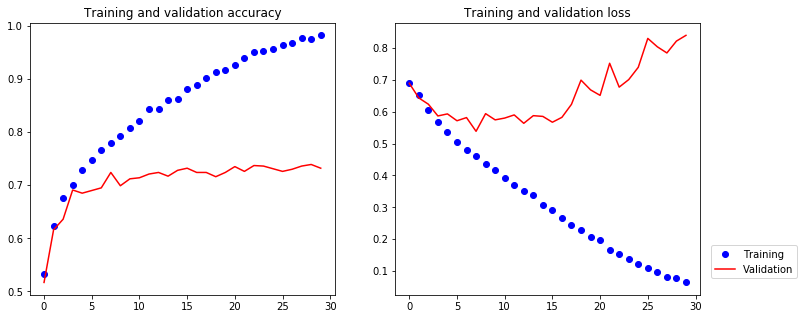
These plots show serious overfitting, because we only have relatively few training samples (2000). We are now going to introduce a technique that can help mitigate overfitting, specific to computer vision, and used almost universally when processing images with deep learning models.

Data Augmentation

Overfitting is caused by having too few samples to learn from, rendering us unable to train a model able to generalize to new data.

Data augmentation takes the approach of generating more training data from existing training samples, by “augmenting” the samples via a number of random transformations that yield believable-looking images. In Keras, this can be done by configuring ImageDataGenerator instance as follows

datagen = image.ImageDataGenerator(rotation_range=40, width_shift_range=0.2,
                             height_shift_range=0.2, shear_range=0.2, zoom_range=0.2,
                             horizontal_flip=True, fill_mode='nearest')

Generation of cat pictures via random data augmentation:

def show_img(index):
    datagen = image.ImageDataGenerator(rotation_range=40, width_shift_range=0.2, height_shift_range=0.2,
                                 shear_range=0.2, zoom_range=0.2, horizontal_flip=True, fill_mode='nearest')

    fnames = [os.path.join(train_cats_dir, fname) for fname in os.listdir(train_cats_dir)]
    # We pick one image to "augment"
    img_path = fnames[index]
    # Read the image and resize it
    img = image.load_img(img_path, target_size=(150, 150))
    # Convert it to a Numpy array with shape (150, 150, 3)
    x = image.img_to_array(img)
    # Reshape it to (1, 150, 150, 3)
    x = x.reshape((1,) + x.shape)
    # The .flow() command below generates batches of randomly transformed images.
    # It will loop indefinitely, so we need to `break` the loop at some point!
    fig = plt.figure(figsize=(10,5))
    for i, batch in enumerate(datagen.flow(x, batch_size=1)):
    #     plt.figure(i)
        plt.subplot(2, 2, i+1)
        imgplot = plt.imshow(image.array_to_img(batch[0]))
        if i % 4 == 3:
            break
    plt.show()
toggle()

show code

interact(show_img, index=widgets.BoundedIntText(min=0,max=100,step=1,value=3,description='Index:'));

To further fight overfitting, we also add a Dropout layer to our model, right before the densely-connected classifier.

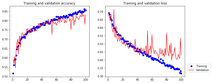
Because of data augmentation and dropout, overfitting is largely mitigated – the training curves are rather closely tracking the validation curves.

def train_model_2():
    model = models.Sequential()
    model.add(layers.Conv2D(32, (3, 3), activation='relu', input_shape=(150, 150, 3)))
    model.add(layers.MaxPooling2D((2, 2)))
    model.add(layers.Conv2D(64, (3, 3), activation='relu'))
    model.add(layers.MaxPooling2D((2, 2)))
    model.add(layers.Conv2D(128, (3, 3), activation='relu'))
    model.add(layers.MaxPooling2D((2, 2)))
    model.add(layers.Conv2D(128, (3, 3), activation='relu'))
    model.add(layers.MaxPooling2D((2, 2)))
    model.add(layers.Flatten())
    model.add(layers.Dropout(0.5))
    model.add(layers.Dense(512, activation='relu'))
    model.add(layers.Dense(1, activation='sigmoid'))
    model.compile(loss='binary_crossentropy',
                  optimizer=optimizers.RMSprop(lr=1e-4),
                  metrics=['acc'])

    train_datagen = image.ImageDataGenerator(rescale=1./255, rotation_range=40, width_shift_range=0.2,
                                       height_shift_range=0.2, shear_range=0.2, zoom_range=0.2,
                                       horizontal_flip=True, fill_mode='nearest')
    # Note that the validation data should not be augmented!
    test_datagen = image.ImageDataGenerator(rescale=1./255)
    train_generator = train_datagen.flow_from_directory(train_dir, target_size=(150, 150),
                                                        batch_size=32, class_mode='binary')
    validation_generator = test_datagen.flow_from_directory(validation_dir, target_size=(150, 150),
                                                            batch_size=32, class_mode='binary')

    history = model.fit_generator(train_generator, steps_per_epoch=100, epochs=100,
                              validation_data=validation_generator, validation_steps=50, verbose=0)
    model.save(base_dir+'\\cats_and_dogs_small_2.h5')
    df = pd.DataFrame.from_dict(data=history.history, orient='columns')
    df.to_csv(base_dir+'\\history_2.csv', header=True, index=False)
    K.clear_session()
    del model
toggle()

show code

df = pd.read_csv(base_dir+'\\history_2.csv')
history = df.to_dict()

acc = list(history['acc'].values())
val_acc = list(history['val_acc'].values())
loss = list(history['loss'].values())
val_loss = list(history['val_loss'].values())
epochs = range(1,len(acc)+1)

plt.figure(figsize=(12, 5))
plt.subplot(1, 2, 1)
plt.plot(epochs, acc, 'bo', label='Training')
plt.plot(epochs, val_acc, 'r', label='Validation')
plt.title('Training and validation accuracy')

plt.subplot(1, 2, 2)
plt.plot(epochs, loss, 'bo', label='Training')
plt.plot(epochs, val_loss, 'r', label='Validation')
plt.title('Training and validation loss')
plt.legend(bbox_to_anchor=(1.02, 0.2), loc=2, borderaxespad=0.5)
plt.show()
toggle()

show code

Although we can continue improving the model, it would be very difficult to have higher accuracy just by training our own convnet from scratch, simply because we have so little data to work with. Next, we will consider a pre-trained model.

Pretrained Convnet

The pre-trained network can effectively act as a generic model of our visual world, and hence its features can prove useful for many different computer vision problems, even though these new problems might involve completely different classes from those of the original task.

The portability of learned features across different problems is a key advantage of deep learning compared to many older shallow learning approaches, and it makes deep learning very effective for small-data problems.

from keras.applications import VGG16
conv_base = VGG16(weights='imagenet', include_top=False, input_shape=(150, 150, 3))

The model is trained on the ImageNet dataset (1.4 million labeled images and 1,000 different classes).

Convnets used for image classification comprise two parts:

• a series of pooling and convolution layers, called the convolutional base of the model, and

• a densely-connected classifier.

In the case of convnets, “feature extraction” will simply consist of taking the convolutional base of a previously-trained network, running the new data through it, and training a new classifier on top of the output.

The option

include_top=False

indicates that we only reuse the convolutional base because the feature maps of a convnet are presence maps of generic concepts over a picture, which is likely to be useful regardless of the computer vision problem at hand.

However, the representations learned by the classifier will necessarily be very specific to the set of classes that the model was trained on – they will only contain information about the presence probability of this or that class in the entire picture.

Additionally, representations found in densely-connected layers no longer contain any information about where objects are located in the input image: these layers get rid of the notion of space, whereas the object location is still described by convolutional feature maps. For problems where object location matters, densely-connected features would be largely useless.

Method 1:

We use a simple densely connected model:

model = models.Sequential()
model.add(layers.Dense(256, activation='relu', input_dim=4 * 4 * 512))
model.add(layers.Dropout(0.5))
model.add(layers.Dense(1, activation='sigmoid'))
model.compile(optimizer=optimizers.RMSprop(lr=2e-5), loss='binary_crossentropy', metrics=['acc'])
model.summary()
toggle()

_________________________________________________________________
Layer (type)                 Output Shape              Param #
=================================================================
dense_3 (Dense)              (None, 256)               2097408
_________________________________________________________________
dropout_1 (Dropout)          (None, 256)               0
_________________________________________________________________
dense_4 (Dense)              (None, 1)                 257
=================================================================
Total params: 2,097,665
Trainable params: 2,097,665
Non-trainable params: 0
_________________________________________________________________

show code

We use pretrained convnet to extract features

features_batch = conv_base.predict(inputs_batch)

The shape of the output feature is (samples, 4, 4, 512) by checking conv_base.summary(). To feed them to a densely-connected classifier, we must flatten them to (samples, 8192).

The flattened outputs are considered as inputs for the densely connected model.

def extract_features(directory, sample_count):
    datagen = image.ImageDataGenerator(rescale=1./255)
    batch_size = 20

    features = np.zeros(shape=(sample_count, 4, 4, 512))
    labels = np.zeros(shape=(sample_count))
    generator = datagen.flow_from_directory(directory, target_size=(150, 150),
                                            batch_size=batch_size, class_mode='binary')
    i = 0
    for inputs_batch, labels_batch in generator:
        features_batch = conv_base.predict(inputs_batch)
        features[i * batch_size : (i + 1) * batch_size] = features_batch
        labels[i * batch_size : (i + 1) * batch_size] = labels_batch
        i += 1
        if i * batch_size >= sample_count:
            # Note that since generators yield data indefinitely in a loop,
            # we must `break` after every image has been seen once.
            break
    return features, labels
toggle()

show code

def pretrained_1():
    model = models.Sequential()
    model.add(layers.Dense(256, activation='relu', input_dim=4 * 4 * 512))
    model.add(layers.Dropout(0.5))
    model.add(layers.Dense(1, activation='sigmoid'))
    model.compile(optimizer=optimizers.RMSprop(lr=2e-5), loss='binary_crossentropy', metrics=['acc'])

    train_features, train_labels = extract_features(train_dir, 2000)
    validation_features, validation_labels = extract_features(validation_dir, 1000)
    test_features, test_labels = extract_features(test_dir, 1000)
    train_features = np.reshape(train_features, (2000, 4 * 4 * 512))
    validation_features = np.reshape(validation_features, (1000, 4 * 4 * 512))
    test_features = np.reshape(test_features, (1000, 4 * 4 * 512))

    history = model.fit(train_features, train_labels, epochs=30, batch_size=20,
                        validation_data=(validation_features, validation_labels), verbose=0)
    df = pd.DataFrame.from_dict(data=history.history, orient='columns')
    df.to_csv(base_dir+'\\history_3.csv', header=True, index=False)
    K.clear_session()
    del model
toggle()

show code

The training results are

df = pd.read_csv(base_dir+'\\history_3.csv')
history = df.to_dict()

acc = list(history['acc'].values())
val_acc = list(history['val_acc'].values())
loss = list(history['loss'].values())
val_loss = list(history['val_loss'].values())
epochs = range(len(acc))

plt.figure(figsize=(12, 5))
plt.subplot(1, 2, 1)
plt.plot(epochs, acc, 'bo', label='Training')
plt.plot(epochs, val_acc, 'r', label='Validation')
plt.title('Training and validation accuracy')

plt.subplot(1, 2, 2)
plt.plot(epochs, loss, 'bo', label='Training')
plt.plot(epochs, val_loss, 'r', label='Validation')
plt.title('Training and validation loss')
plt.legend(bbox_to_anchor=(1.02, 0.2), loc=2, borderaxespad=0.5)
plt.show()
toggle()

show code

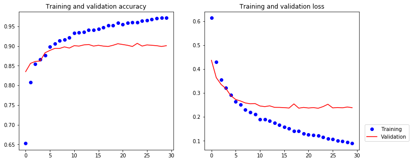
The model has a validation accuracy of about 90%, much better than our small model trained from scratch. However, our plots also indicate that we are overfitting almost from the start – despite using dropout with a fairly large rate. This is because this technique does not leverage data augmentation, which is essential to preventing overfitting with small image datasets.

---

Method 2:

A better approach is to add pretrained convnet into our model

model.add(conv_base)

then we will fit this new model with augmented data. To take the advantage of the pretrained model, we freeze its weights

conv_base.trainable = False

As shown in the model summary, the parameters in our convolution base are untrainable.

model = models.Sequential()
model.add(conv_base)
model.add(layers.Flatten())
model.add(layers.Dense(256, activation='relu'))
model.add(layers.Dense(1, activation='sigmoid'))
conv_base.trainable = False
model.summary()
toggle()

_________________________________________________________________
Layer (type)                 Output Shape              Param #
=================================================================
vgg16 (Model)                (None, 4, 4, 512)         14714688
_________________________________________________________________
flatten_2 (Flatten)          (None, 8192)              0
_________________________________________________________________
dense_5 (Dense)              (None, 256)               2097408
_________________________________________________________________
dense_6 (Dense)              (None, 1)                 257
=================================================================
Total params: 16,812,353
Trainable params: 2,097,665
Non-trainable params: 14,714,688
_________________________________________________________________

show code

We can use data-augmentation configuration and train the model

train_datagen = image.ImageDataGenerator(rescale=1./255, rotation_range=40, width_shift_range=0.2,
                                   height_shift_range=0.2, shear_range=0.2, zoom_range=0.2,
                                   horizontal_flip=True, fill_mode='nearest')
test_datagen = image.ImageDataGenerator(rescale=1./255)
train_generator = train_datagen.flow_from_directory(train_dir, target_size=(150, 150),
                                                    batch_size=20, class_mode='binary')
validation_generator = test_datagen.flow_from_directory(validation_dir, target_size=(150, 150),
                                                        batch_size=20, class_mode='binary')
model.compile(loss='binary_crossentropy', optimizer=optimizers.RMSprop(lr=2e-5), metrics=['acc'])

def pretrained_2():
    history = model.fit_generator(train_generator, steps_per_epoch=100, epochs=30,
                              validation_data=validation_generator, validation_steps=50, verbose=0)
    model.save(base_dir+'\\cats_and_dogs_small_3.h5')
    df = pd.DataFrame.from_dict(data=history.history, orient='columns')
    df.to_csv(base_dir+'\\history_4.csv', header=True, index=False)
toggle()

Found 2000 images belonging to 2 classes.
Found 1000 images belonging to 2 classes.

show code

df = pd.read_csv(base_dir+'\\history_4.csv')
history = df.to_dict()

acc = list(history['acc'].values())
val_acc = list(history['val_acc'].values())
loss = list(history['loss'].values())
val_loss = list(history['val_loss'].values())
epochs = range(len(acc))

plt.figure(figsize=(12, 5))
plt.subplot(1, 2, 1)
plt.plot(epochs, acc, 'bo', label='Training')
plt.plot(epochs, val_acc, 'r', label='Validation')
plt.title('Training and validation accuracy')

plt.subplot(1, 2, 2)
plt.plot(epochs, loss, 'bo', label='Training')
plt.plot(epochs, val_loss, 'r', label='Validation')
plt.title('Training and validation loss')
plt.legend(bbox_to_anchor=(1.02, 0.2), loc=2, borderaxespad=0.5)
plt.show()
toggle()

show code

Note that the level of generality (and therefore reusability) of the representations extracted by specific convolution layers depends on the depth of the layer in the model.

• Layers that come earlier in the model extract local, highly generic feature maps (such as visual edges, colors, and textures), while

• layers higher-up extract more abstract concepts (such as “cat ear” or “dog eye”).

If our new dataset differs a lot from the dataset that the original model was trained on, we may be better off using only the first few layers of the model to do feature extraction, rather than using the entire convolutional base.

For example, we can fine-tuning the top layers above layer “block5_conv1” with following a few lines of codes.

conv_base.trainable = True
set_trainable = False
for layer in conv_base.layers:
    if layer.name == 'block5_conv1':
        set_trainable = True
    if set_trainable:
        layer.trainable = True
    else:
        layer.trainable = False

We can evaluate a model on the test data:

model = models.load_model(base_dir+"\\cats_and_dogs_small_3.h5")
test_generator = test_datagen.flow_from_directory(test_dir, target_size=(150, 150), batch_size=20, class_mode='binary')
test_loss, test_acc = model.evaluate_generator(test_generator, steps=50)
print('test acc:', test_acc)

Found 1000 images belonging to 2 classes.
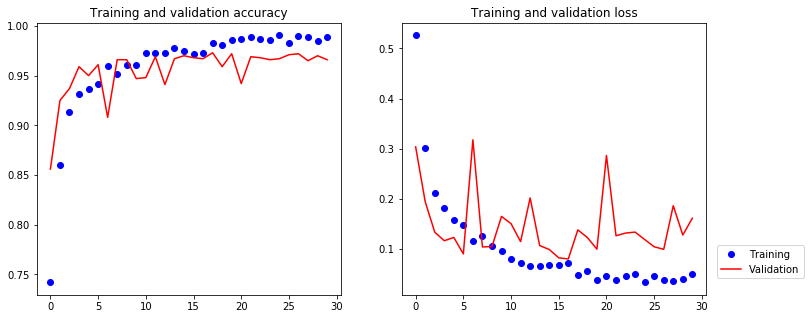
test acc: 0.9659999918937683

Visualizing the Convnets

The representations learned by convnets are highly amenable to visualization, in large part because they are representations of visual concepts

Intermediate Activations

We load an cat image and create an image tensor with shape (1, 150, 150, 3) where 1 indicates one image, 150 \(\times\) 150 is the image size, 3 is the color depth.

Then, we extracts the outputs of the top 8 layers

layer_outputs = [layer.output for layer in model.layers[:8]]

and initiate a model return these outputs when input is given

activation_model = models.Model(inputs=model.input, outputs=layer_outputs)

If we give an image tensor as input for prediction,

activations = activation_model.predict(an image tensor)

activations returns a list of 8 numpy arrays. Each array has shape (1, 148, 148, 32) which is a 148 \(\times\) 148 feature map with 32 channels.

def show_catimg(imgidx, channel):
    img_path = test_cats_dir + "\\cat.{}.jpg".format(imgidx)
    img = image.load_img(img_path, target_size=(150, 150))
    img_tensor = image.img_to_array(img)
    img_tensor = np.expand_dims(img_tensor, axis=0)
    # Remember that the model was trained on inputs
    # that were preprocessed in the following way:
    img_tensor /= 255.
    plt.imshow(img_tensor[0])
    plt.show()

    model = models.load_model(base_dir+'\\cats_and_dogs_small_2.h5')
    layer_outputs = [layer.output for layer in model.layers[:8]]
    activation_model = models.Model(inputs=model.input, outputs=layer_outputs)
    activations = activation_model.predict(img_tensor)
    fig, axes = plt.subplots(1, min(5, 32-channel), figsize=(20, 5))
    for i in range(min(5, 32-channel)):
        axes[i].set_title('First layer channel {}'.format(channel+i), pad=15)
        axes[i].matshow(activations[0][0,:,:,channel+i], cmap='viridis')
toggle()

show code

interact(show_catimg, imgidx=widgets.BoundedIntText(min=1500,max=1900,step=1,value=1700,description='Image:'),
         channel=widgets.BoundedIntText(min=0,max=31,step=1,value=4,description='Channel:'));

The first few layers acts as a collection of various edge detectors. At that stage, the activations are still retaining almost all of the information present in the initial picture. The activations become increasingly abstract and less visually interpretable. The sparsity of the activations is increasing with the depth of the layer as we see more black feature maps. Because more and more filters are blank, the pattern encoded by the filter isn’t found in the input image.

A deep neural network effectively acts as an information distillation pipeline, with raw data going in (in our case, RBG pictures), and getting repeatedly transformed so that irrelevant information gets filtered out (e.g. the specific visual appearance of the image) while useful information get magnified and refined (e.g. the class of the image).

def show_imglayer(imgidx, layer_name):
    img_path = test_cats_dir + "\\cat.{}.jpg".format(imgidx)
    img = image.load_img(img_path, target_size=(150, 150))
    img_tensor = image.img_to_array(img)
    img_tensor = np.expand_dims(img_tensor, axis=0)
    # Remember that the model was trained on inputs
    # that were preprocessed in the following way:
    img_tensor /= 255.
    plt.imshow(img_tensor[0])

    layer_outputs = [layer.output for layer in model.layers[:8]]
    activation_model = models.Model(inputs=model.input, outputs=layer_outputs)
    activations = activation_model.predict(img_tensor)

    layer_names = [layer.name for layer in model.layers[:8]]

    images_per_row = 16
    layer_activation = activations[layer_names.index(layer_name)]

    # This is the number of features in the feature map
    n_features = layer_activation.shape[-1]

    # The feature map has shape (1, size, size, n_features)
    size = layer_activation.shape[1]

    # We will tile the activation channels in this matrix
    n_cols = n_features // images_per_row
    display_grid = np.zeros((size * n_cols, images_per_row * size))

    # We'll tile each filter into this big horizontal grid
    for col in range(n_cols):
        for row in range(images_per_row):
            channel_image = layer_activation[0,
                                             :, :,
                                             col * images_per_row + row]
            # Post-process the feature to make it visually palatable
            channel_image -= channel_image.mean()
            channel_image /= channel_image.std()
            channel_image *= 64
            channel_image += 128
            channel_image = np.clip(channel_image, 0, 255).astype('uint8')
            display_grid[col * size : (col + 1) * size,
                         row * size : (row + 1) * size] = channel_image

    # Display the grid
    scale = 1. / size
    plt.figure(figsize=(scale * display_grid.shape[1],
                        scale * display_grid.shape[0]))
    plt.title(layer_name)
    plt.grid(False)
    plt.imshow(display_grid, aspect='auto', cmap='viridis')

    plt.show()
toggle()

show code

model = models.load_model(base_dir+'\\cats_and_dogs_small_2.h5')
layer_names = [layer.name for layer in model.layers[:8]]
interact(show_imglayer,
         imgidx=widgets.BoundedIntText(min=1500,max=1900,step=1,value=1700,description='Image:'),
         layer_name=widgets.Dropdown(options=layer_names, value='conv2d_5', description='Layer:',disabled=False));

Convnet Filters

In neural network terminology, the learned filters are simply weights. Consider the conv2d_5 layer. The filter has shape (3, 3, 3, 32) where it has dimension 3 \(\times\) 3 (first two “3”s), 3 input depth and 32 output depth.

def deprocess_image(x):
    # normalize tensor: center on 0., ensure std is 0.1
    x -= x.mean()
    x /= (x.std() + 1e-5)
    x *= 0.1

    # clip to [0, 1]
    x += 0.5
    x = np.clip(x, 0, 1)

    # convert to RGB array
    x *= 255
    x = np.clip(x, 0, 255).astype('uint8')
    return x

def filters(idx):
    layer_name = 'conv2d_5'
    filters, biases = model.get_layer(layer_name).get_weights()
    f_min, f_max = filters.min(), filters.max()
    filters = (filters - f_min) / (f_max - f_min)
    fig, axes =  plt.subplots(3, 5, figsize=(15, 6))
    cols = ['Out Depth {}'.format(col+idx) for col in range(5)]
    rows = ['Input Depth {}'.format(row) for row in range(3)]
    for ax, col in zip(axes[0], cols):
        ax.set_title(col)
    for ax, row in zip(axes[:,0], rows):
        ax.set_ylabel(row, rotation=0, size='large')
        ax.yaxis.set_label_coords(-.6,.4)
    for i in range(3):
        for j in range(5):
            axes[i,j].imshow(filters[:, :, i, idx+j])
    fig.tight_layout()
    plt.show()
toggle()

show code

model = models.load_model(base_dir+'\\cats_and_dogs_small_2.h5')
interact(filters, idx=widgets.BoundedIntText(min=0,max=31,step=1,value=0,description='Depth:'));

We can also apply each filter to a blank input image (gray image with some noise)

input_img_data = np.zeros((1, 150, 150, 3)) * 20 + 128
plt.figure(figsize=(3, 3))
plt.imshow(deprocess_image(input_img_data[0]))
plt.show()

By using gradient ascent (as the opposite of gradient descent), we try to maximize the effect of a filter. The resulting image would be one that the chosen filter is maximally responsive to.

def generate_pattern(layer_name, filter_index, size=150):
    # Build a loss function that maximizes the activation
    # of the nth filter of the layer considered.
    layer_output = model.get_layer(layer_name).output
    loss = K.mean(layer_output[:, :, :, filter_index])

    # Compute the gradient of the input picture wrt this loss
    grads = K.gradients(loss, model.input)[0]

    # Normalization trick: we normalize the gradient
    grads /= (K.sqrt(K.mean(K.square(grads))) + 1e-5)

    # This function returns the loss and grads given the input picture
    iterate = K.function([model.input], [loss, grads])

    # We start from a gray image with some noise
    input_img_data = np.random.random((1, size, size, 3)) * 20 + 128.

    # Run gradient ascent for 40 steps
    step = 1.
    for i in range(20):
        loss_value, grads_value = iterate([input_img_data])
        input_img_data += grads_value * step

    img = input_img_data[0]
    return deprocess_image(img)

def show_filters(layer_name):
    size = 64
    margin = 5
    layout = 3

    results = np.zeros((layout * size + (layout-1) * margin, layout * size + (layout-1) * margin, 3))
    for i in range(layout):  # iterate over the rows of our results grid
        for j in range(layout):  # iterate over the columns of our results grid
            filter_img = generate_pattern(layer_name, i + (j * layout), size=size)
            horizontal_start = i * size + i * margin
            horizontal_end = horizontal_start + size
            vertical_start = j * size + j * margin
            vertical_end = vertical_start + size
            results[horizontal_start: horizontal_end, vertical_start: vertical_end, :] = filter_img

    plt.figure(figsize=(10, 10))
    plt.imshow(deprocess_image(results))
    plt.show()
toggle()

show code

# model = models.load_model(base_dir+'\\cats_and_dogs_small_2.h5')
# layer_names = ['conv2d_5', 'conv2d_6', 'conv2d_7', 'conv2d_8']
model = VGG16(weights='imagenet', include_top=False)
layer_names = ['block1_conv1', 'block2_conv1', 'block3_conv1', 'block4_conv1']
interact(show_filters,
         layer_name=widgets.Dropdown(options=layer_names, value=layer_names[-1], description='Layer:',disabled=False));

These filter visualizations tell us how convnet layers see the world. Each layer in a convnet simply learns a collection of filters such that their inputs can be expressed as a combination of the filters.

The filters from the first layer usually encode simple directional edges and colors. The filters in higher-up layers start resembling textures found images.

Heatmaps of Class Activation

This techniques is called “Class Activation Map” (CAM) visualization, and consists in producing heatmaps of “class activation” over input images. We demonstrate this technique using the VGG16 network with the densely-connected classifier on top (we drop option include_top=False).

model = VGG16(weights='imagenet')

We process the image and use VGG16 to predict it.

from keras.applications.vgg16 import preprocess_input, decode_predictions
img = image.load_img(base_dir+'\\creative_commons_elephant.jpg', target_size=(224, 224))
x = image.img_to_array(img) # `x` is a float32 Numpy array of shape (224, 224, 3)
x = np.expand_dims(x, axis=0) # `x` is a float32 Numpy array of shape (1, 224, 224, 3)
x = preprocess_input(x)
preds = model.predict(x) # with shape (1, 1000)
print('argmax(preds):', np.argmax(preds[0]))
print('Predicted:', decode_predictions(preds, top=3)[0])

argmax(preds): 386
Predicted: [('n02504458', 'African_elephant', 0.90942156), ('n01871265', 'tusker', 0.08618244), ('n02504013', 'Indian_elephant', 0.004354585)]

The top-3 classes predicted for this image are:

• African elephant (with 92.5% probability)

• Tusker (with 7% probability)

• Indian elephant (with 0.4% probability)

The entry in the prediction vector that was maximally activated is the one corresponding to the “African elephant” class, at index 386:

# This is the "african elephant" entry in the prediction vector
african_elephant_output = model.output[:, 386]

# The is the output feature map of the `block5_conv3` layer,
# the last convolutional layer in VGG16
last_conv_layer = model.get_layer('block5_conv3')

# This is the gradient of the "african elephant" class with regard to
# the output feature map of `block5_conv3`
grads = K.gradients(african_elephant_output, last_conv_layer.output)[0]

# This is a vector of shape (512,), where each entry
# is the mean intensity of the gradient over a specific feature map channel
pooled_grads = K.mean(grads, axis=(0, 1, 2))

# This function allows us to access the values of the quantities we just defined:
# `pooled_grads` and the output feature map of `block5_conv3`,
# given a sample image
iterate = K.function([model.input], [pooled_grads, last_conv_layer.output[0]])

# These are the values of these two quantities, as Numpy arrays,
# given our sample image of two elephants
pooled_grads_value, conv_layer_output_value = iterate([x])

# We multiply each channel in the feature map array
# by "how important this channel is" with regard to the elephant class
for i in range(512):
    conv_layer_output_value[:, :, i] *= pooled_grads_value[i]

# The channel-wise mean of the resulting feature map
# is our heatmap of class activation
heatmap = np.mean(conv_layer_output_value, axis=-1)
heatmap = np.maximum(heatmap, 0)
heatmap /= np.max(heatmap)
plt.matshow(heatmap)
plt.show()

import cv2
img = cv2.imread(base_dir+"\\creative_commons_elephant.jpg")
heatmap = cv2.resize(heatmap, (img.shape[1], img.shape[0]))
heatmap = np.uint8(255 * heatmap) # convert the heatmap to RGB
heatmap = cv2.applyColorMap(heatmap, cv2.COLORMAP_JET) # apply the heatmap to the original image
superimposed_img = heatmap * 0.4 + img # 0.4 here is a heatmap intensity factor
# cv2.imwrite(base_dir+'\\elephant_cam.jpg', superimposed_img)
plt.figure(figsize=(10, 10))
plt.imshow(deprocess_image(superimposed_img))
plt.show()
toggle()

show code

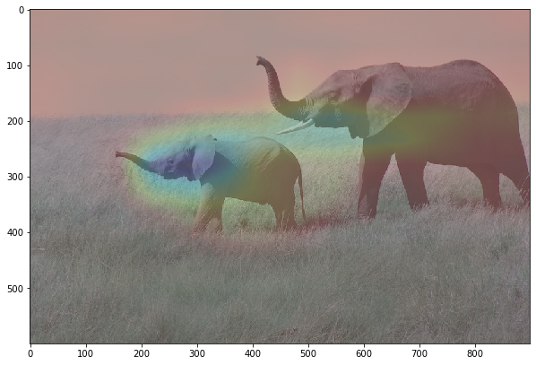
This visualisation technique answers two important questions:

• Why did the network think this image contained an African elephant?

• Where is the African elephant located in the picture?

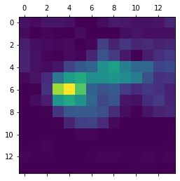
In particular, it is interesting to note that the ears of the elephant cub are strongly activated: this is probably how the network can tell the difference between African and Indian elephants.

This is helpful for “debugging” the decision process of a convnet, in particular in case of a classification mistake. It also allows you to locate specific objects in an image.

Deep Dream

We use Inception V3 model and disable all training-specific operations.

from keras.applications import inception_v3
K.set_learning_phase(0)
model = inception_v3.InceptionV3(weights='imagenet', include_top=False)

def resize_img(img, size):
    import scipy
    img = np.copy(img)
    factors = (1,
               float(size[0]) / img.shape[1],
               float(size[1]) / img.shape[2],
               1)
    return scipy.ndimage.zoom(img, factors, order=1)

def preprocess_image(image_path):
    if image_path.startswith('http://') or image_path.startswith('https://'):
        import requests
        from io import BytesIO
        from PIL import Image
        response = requests.get(image_path)
        img = Image.open(BytesIO(response.content))
    else:
        img = image.load_img(image_path)
    img = image.img_to_array(img)
    img = np.expand_dims(img, axis=0)
    img = inception_v3.preprocess_input(img)
    return img

def deprocess_image(x):
    # Util function to convert a tensor into a valid image.
    if K.image_data_format() == 'channels_first':
        x = x.reshape((3, x.shape[2], x.shape[3]))
        x = x.transpose((1, 2, 0))
    else:
        x = x.reshape((x.shape[1], x.shape[2], 3))
    x /= 2.
    x += 0.5
    x *= 255.
    x = np.clip(x, 0, 255).astype('uint8')
    return x
toggle()

show code

For the filter visualization, we try to maximize the value of a specific filter in a specific layer. Here, we simultaneously maximize the activation of all filters in a number of layers.

We define a set of coefficients quantifying how much the layer’s activation contributes to the loss we will maximize.

The loss is defined as L2 norm (sum of squares) of activation activation[:, 2: -2, 2: -2, :] for all batches, only non-border pixels, and all channels.

layer_contributions = {
    'mixed2': 0.2,
    'mixed3': 3.,
    'mixed4': 2.,
    'mixed5': 1.5,
}

layer_dict = dict([(layer.name, layer) for layer in model.layers])

loss = K.variable(0.)
for layer_name in layer_contributions:
    coeff = layer_contributions[layer_name]
    activation = layer_dict[layer_name].output
    scaling = K.prod(K.cast(K.shape(activation), 'float32'))
    loss = loss + coeff * K.sum(K.square(activation[:, 2: -2, 2: -2, :])) / scaling

dream = model.input

grads = K.gradients(loss, dream)[0]
grads /= K.maximum(K.mean(K.abs(grads)), 1e-7) # Normalize gradients.

outputs = [loss, grads]
fetch_loss_and_grads = K.function([dream], outputs)

def eval_loss_and_grads(x):
    outs = fetch_loss_and_grads([x])
    loss_value = outs[0]
    grad_values = outs[1]
    return loss_value, grad_values

def gradient_ascent(x, iterations, step, max_loss=None):
    for i in range(iterations):
        loss_value, grad_values = eval_loss_and_grads(x)
        if max_loss is not None and loss_value > max_loss:
            break
        if i % 5==0:
            print('...Loss value at', i, ':', loss_value)
        x += step * grad_values
    return x

The loss value keeps increasing as we are maximizing filters effects. If our loss gets larger than 10, we will interrupt the gradient ascent process, to avoid ugly artifacts.

def deepdream(img_path):
    # Playing with these hyperparameters will also allow you to achieve new effects
    step = 0.01  # Gradient ascent step size
    num_octave = 3  # Number of scales at which to run gradient ascent
    octave_scale = 1.4  # Size ratio between scales
    iterations = 20  # Number of ascent steps per scale

    max_loss = 10
    img = preprocess_image(img_path)
    original_shape = img.shape[1:3]
    original_img = np.copy(img)
    shape = tuple([int(dim / (max(original_shape)/400)) for dim in original_shape])
    shrunk_original_img = resize_img(img, shape)
    img = resize_img(img, shape)
    img = gradient_ascent(img,
                          iterations=iterations,
                          step=step,
                          max_loss=max_loss)
    upscaled_shrunk_original_img = resize_img(shrunk_original_img, shape)
    same_size_original = resize_img(original_img, shape)
    lost_detail = same_size_original - upscaled_shrunk_original_img

    img += lost_detail
    shrunk_original_img = resize_img(original_img, shape)

    plt.figure(figsize=(10, 10))
    plt.imshow(deprocess_image(np.copy(original_img)))
    plt.figure(figsize=(10, 10))
    plt.imshow(deprocess_image(np.copy(img)))
    plt.show()

toggle()

show code

interact(deepdream,
         img_path=widgets.Text(value='https://cdn.abcotvs.com/dip/images/1904036_042217-ktrk-buffalo-bayou-cover-img.jpg?w=800&r=16%3A9',
                               placeholder='Type something', description='URL:', disabled=False));

Neural Style Transfer

from keras.applications import vgg19
content_image_path = "https://raw.githubusercontent.com/ming-zhao/Optimization-and-Learning/master/figures/portrait.png"
style_image_path = "https://raw.githubusercontent.com/ming-zhao/Optimization-and-Learning/master/figures/popova.png"

response = requests.get(content_image_path)
img = Image.open(BytesIO(response.content))

width, height = img.size
img_height = 400
img_width = int(width * img_height / height)

def preprocess_image(image_path):
    response = requests.get(image_path)
    img = Image.open(BytesIO(response.content)).resize((img_width, img_height))
    img = image.img_to_array(img)
    img = np.expand_dims(img, axis=0)
    img = vgg19.preprocess_input(img)
    return img[:,:,:,:3]

def deprocess_image(x):
    # Remove zero-center by mean pixel
    x[:, :, 0] += 103.939
    x[:, :, 1] += 116.779
    x[:, :, 2] += 123.68
    # 'BGR'->'RGB'
    x = x[:, :, ::-1]
    x = np.clip(x, 0, 255).astype('uint8')
    return x

content_image = K.constant(preprocess_image(content_image_path))
style_image = K.constant(preprocess_image(style_image_path))
generated_image = K.placeholder((1, img_height, img_width, 3))
input_tensor = K.concatenate([content_image, style_image, generated_image], axis=0)
toggle()

show code

Neural style transfer consists in applying the “style” of a reference image to a target image, while conserving the “content” of the target image.

If we were able to mathematically define content and style, then an appropriate loss function to minimize would be the following:

loss = distance(style(style_image) - style(generated_image)) +
       distance(content(content_image) - content(generated_image))

where distance is a norm function such as the L2 norm, content is a function that takes an image and computes a representation of its “content”, and style is a function that takes an image and computes a representation of its “style”.

Recall that activations from earlier layers in a network contain local information about the image, while activations from higher layers contain increasingly global and abstract information. The content loss only leverages a single higher-up layer.

While the content loss only leverages a single higher-up layer, the style loss as defined in the Gatys et al. paper leverages multiple layers of a convnet: we aim at capturing the appearance of the style reference image at all spatial scales extracted by the convnet, not just any single scale.

The style loss leverages the “Gram matrix” of a layer’s activations, i.e. the inner product between the feature maps of a given layer \(X X^\intercal\). This inner product can be understood as representing a map of the correlations between the features of a layer. These feature correlations capture the statistics of the patterns of a particular spatial scale, which empirically corresponds to the appearance of the textures found at this scale.

def content_loss(content, generated):
    return K.sum(K.square(generated - content))

def gram_matrix(x):
    features = K.batch_flatten(K.permute_dimensions(x, (2, 0, 1)))
    gram = K.dot(features, K.transpose(features))
    return gram

def style_loss(style, generated):
    S = gram_matrix(style)
    C = gram_matrix(generated)
    channels = 3
    size = img_height * img_width
    return K.sum(K.square(S - C)) / (4. * (channels ** 2) * (size ** 2))

def total_variation_loss(x):
    a = K.square(
        x[:, :img_height - 1, :img_width - 1, :] - x[:, 1:, :img_width - 1, :])
    b = K.square(
        x[:, :img_height - 1, :img_width - 1, :] - x[:, :img_height - 1, 1:, :])
    return K.sum(K.pow(a + b, 1.25))


model = vgg19.VGG19(input_tensor=input_tensor, weights='imagenet', include_top=False)

total_variation_weight = 1e-4
style_weight = 1.
content_weight = 0.025

outputs_dict = dict([(layer.name, layer.output) for layer in model.layers])
content_layer = 'block5_conv2'
style_layers = ['block1_conv1',
                'block2_conv1',
                'block3_conv1',
                'block4_conv1',
                'block5_conv1']

loss = K.variable(0.)
layer_features = outputs_dict[content_layer]
content_features = layer_features[0, :, :, :]
generated_features = layer_features[2, :, :, :]
loss = loss + content_weight * content_loss(content_features, generated_features)

for layer_name in style_layers:
    layer_features = outputs_dict[layer_name]
    style_features = layer_features[1, :, :, :]
    generated_features = layer_features[2, :, :, :]
    sl = style_loss(style_features, generated_features)
    loss = loss + (style_weight / len(style_layers)) * sl
loss = loss + total_variation_weight * total_variation_loss(generated_image)

toggle()

show code

from scipy.optimize import fmin_l_bfgs_b

class Evaluator(object):

    def __init__(self):
        self.loss_value = None
        self.grads_values = None

    def loss(self, x):
        assert self.loss_value is None
        x = x.reshape((1, img_height, img_width, 3))
        grads = K.gradients(loss, generated_image)[0]
        fetch_loss_and_grads = K.function([generated_image], [loss, grads])
        outs = fetch_loss_and_grads([x])
        loss_value = outs[0]
        grad_values = outs[1].flatten().astype('float64')
        self.loss_value = loss_value
        self.grad_values = grad_values
        return self.loss_value

    def grads(self, x):
        assert self.loss_value is not None
        grad_values = np.copy(self.grad_values)
        self.loss_value = None
        self.grad_values = None
        return grad_values

evaluator = Evaluator()
x = preprocess_image(content_image_path).flatten()
for i in range(0):
    print('Start of iteration', i)
    start_time = time.time()
    x, min_val, info = fmin_l_bfgs_b(evaluator.loss, x,
                                     fprime=evaluator.grads, maxfun=20)
    print('Current loss value:', min_val)
    img = x.copy().reshape((img_height, img_width, 3))
    img = deprocess_image(img)
    fname = base_dir + '\\style_transfer_result_at_iteration_%d.png' % i
    cv2.imwrite(fname, img)
    end_time = time.time()
    print('Image saved as', fname)
    print('Iteration %d completed in %ds' % (i, end_time - start_time))

toggle()

show code