%run ../initscript.py
import pandas as pd
import numpy as np
import matplotlib.pyplot as plt
import matplotlib
from ipywidgets import *
import pandas as pd
%matplotlib inline

import sys
sys.path.append('modules')

from DesignMat import Polynomial
from Classifier import LeastSquares, Logistic

from sklearn.linear_model import LinearRegression, LogisticRegression, BayesianRidge
from sklearn.discriminant_analysis import LinearDiscriminantAnalysis, QuadraticDiscriminantAnalysis

toggle()

show code

Linear Models for Classification

We introduce 3 training datasets that will be used in this note.

np.random.seed(12321)
x0 = np.random.normal(size=50).reshape(-1, 2) - 1
x1 = np.random.normal(size=50).reshape(-1, 2) + 1
x2 = np.random.normal(size=50).reshape(-1, 2) + 3.
x_1 = np.random.normal(size=10).reshape(-1, 2) + np.array([11., 10.])

train_data ={'2-class': (np.concatenate([x0, x1]), np.concatenate([np.zeros(25), np.ones(25)]).astype(np.int)),
             '2-class_ex':
             (np.concatenate([x0, x1, x_1]), np.concatenate([np.zeros(25), np.ones(30)]).astype(np.int)),
             '3-class':
             (np.concatenate([x0, x1, x2]), np.concatenate([np.zeros(25), np.ones(25), 2 + np.zeros(25)]).astype(np.int))}

plt.figure(figsize=(15, 4))
for i, (key, value) in enumerate(train_data.items()):
    plt.subplot(1, 3, i+1)
    x_train, t_train = value
    plt.scatter(x_train[:,0], x_train[:,1], c=t_train, cmap=matplotlib.colors.ListedColormap(['red','green','blue']))
    plt.title("{}".format(key))
plt.show()

toggle()

show code

The goal in classification is to assign \(p\)-dimension \(\mathbf{x}\) to one of \(K\) classes \(\mathcal{C}_k\). In general, there are two approaches to perform the task:

• Nonprobabilistic approach constructs a discriminant function that directly assigns each vector \(\mathbf{x}\) to a specific class.

• Probabilistic approach models the conditional probability distribution \(p(\mathcal{C}_k|\mathbf{x})\) in an inference stage, and then subsequently uses this distribution to make optimal decisions.

We define target vector as

\begin{align*} \mathbf{t} = (t_k: k = 1, \ldots, K)^\intercal \end{align*}

where the value of \(t_k\) is interpreted as the probability that the class is \(\mathcal{C}_k\). For example, \(\mathbf{t} = (0, 1, 0, 0, 0)^\intercal\) indicates a pattern from class 2 out of 5 classes.

Discriminant Functions

When \(K=2\), consider a linear discriminant function \(y(\mathbf{x}) = \mathbf{w}^\intercal \mathbf{x} + w_0\) assigns \(\mathbf{x}\) to

• class \(\mathcal{C}_1\) if \(y(\mathbf{x}) \ge 0\), and

• class \(\mathcal{C}_2\) otherwise.

where \(\mathbf{w}\) is called a weight vector, and \(w_0\) is a bias. The negative of the bias is sometimes called a threshold.

When \(K>2\), it is tempting to build a \(K\)-class discriminant by combining two-class functions.

• One-versus-the-rest: \(K-1\) classifiers each of which solves a two-class problem of separating points in a particular class \(\mathcal{C}_k\) from points not in that class.

• One-versus-one: \(K(K-1)/2\) binary discriminant functions, one for every possible pair of classes.

• Both approach lead to regions of input space that are ambiguously classified.

A single \(K\)-class discriminant comprising \(K\) linear functions of the form:

\begin{align*} y_k(\mathbf{x}) = \mathbf{w}_k^\intercal \mathbf{x} + w_{k0} \end{align*}

\(\mathbf{x}\) is assigned to class \(\mathcal{C}_{k^\ast}\) if \(y_{k^\ast}(\mathbf{x}) > y_j(\mathbf{x})\) for all \(j \ne k^\ast\), i.e. class

\begin{align*} k^* = \text{argmax}_k \{y_k(\mathbf{x}): k = 1,\ldots,K\} \end{align*}

Least Squares

Consider a training data set \(\{\mathbf{x}_i, \mathbf{t}_i\}\) where \(i = 1,\ldots,n\). The least squares approach is to find \(\mathbf{w}_k\), \(k = 1, \ldots, K\) such that

the sum-of-squares error between \(\mathbf{y}(\mathbf{x_i}) = (y_1(\mathbf{x}), \ldots, y_K(\mathbf{x}))\) and \(\mathbf{t}_i\) is minimal.

• The least squares is equivalent to maximum likelihood of a Gaussian conditional distribution (\(p(y|\mathbf{x}, \mathbf{w}, \beta) = \mathcal{N}(y | f(\mathbf{x}, \mathbf{w}), \beta^{-1})\)),

• However, binary target vectors clearly have a distribution that is far from Gaussian.

• When, for most of \(\mathbf{x} \in \mathcal{C}_k\), there always exists \(j\) such that \(y_{k}(\mathbf{x}) < y_j(\mathbf{x})\) for many, class \(\mathcal{C}_k\) is masked by others because the nature of linear function.

hide_comment()

show comment

Least squares solution

We can conveniently group those linear models together using vector notation so that \begin{align} \mathbf{y}(\mathbf{x}) = \tilde{\mathbf{W}}^T \tilde{\mathbf{x}} \nonumber \end{align}

where

\begin{align} \tilde{\mathbf{W}} = \left( \begin{array}{lll} w_{10} & \cdots & w_{K0} \\ \mathbf{w}_1^\intercal & \cdots & \mathbf{w}_K^\intercal \end{array} \right) = \left( \begin{array}{lll} w_{10} & \cdots & w_{K0} \\ w_{11} & \cdots & w_{K1} \\ \vdots & \ddots & \vdots \\ w_{1d} & \cdots & w_{Kd} \\ \end{array} \right)_{(p+1) \times K},~ \tilde{\mathbf{x}} = \left( \begin{array}{l} 1 \\ x_{1} \\ \vdots \\ x_{p} \\ \end{array} \right) \nonumber \end{align}

Consider a training data set \(\{\mathbf{x}_i, \mathbf{t}_i\}\) where \(i = 1,\ldots,n\) and define

\begin{align} \mathbf{T} = \left( \begin{array}{l} \mathbf{t}_1 \\ \mathbf{t}_2 \\ \vdots \\ \mathbf{t}_n \\ \end{array} \right)_{n \times K} \text{ and } \tilde{\mathbf{X}} = \left( \begin{array}{l} \tilde{\mathbf{x}}^\intercal_1 \\ \tilde{\mathbf{x}}^\intercal_2 \\ \vdots \\ \tilde{\mathbf{x}}^\intercal_n \\ \end{array} \right)_{n \times (p+1)} \nonumber \end{align}

where \(\mathbf{t}_i = (0, \ldots, 0, \underbrace{1}_{k}, 0, \ldots, 0 )_{K \times 1}\) indicates \(\mathbf{x}_i \in k\)-class. Minimizing the sum-of-squares error function

\begin{align} \mathbb{SSE} \left[ \tilde{\mathbf{W}} \right] = \frac{1}{2} \text{Tr} \left\{ \left( \tilde{\mathbf{X}}\tilde{\mathbf{W}} - \mathbf{T}\right)^\intercal \left( \tilde{\mathbf{X}}\tilde{\mathbf{W}} - \mathbf{T}\right) \right\} \text{ gives } \tilde{\mathbf{W}} = \left( \tilde{\mathbf{X}}^\intercal \tilde{\mathbf{X}} \right)^{-1} \tilde{\mathbf{X}}^\intercal \mathbf{T} \nonumber \end{align}

\(\blacksquare\)

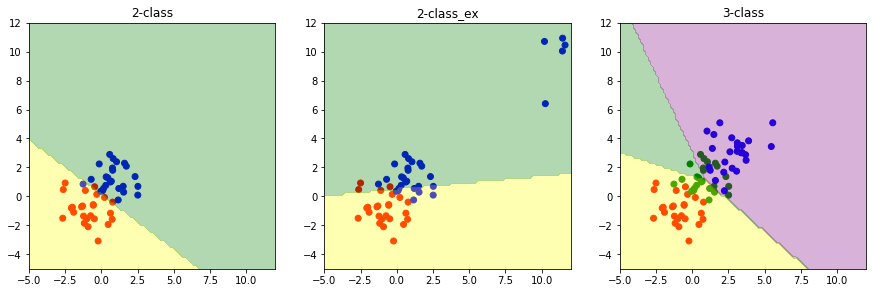
The plots demonstrate the least squares method for classification.

x1_test, x2_test = np.meshgrid(np.linspace(-5, 12, 100), np.linspace(-5, 12, 100))
x_test = np.array([x1_test, x2_test]).reshape(2, -1).T

plt.figure(figsize=(15, 5))
for i, (key, value) in enumerate(train_data.items()):
    plt.subplot(1, 3, i+1)
    x_train, t_train = value
    t = LeastSquares().fit(x_train, t_train).predict(x_test)
    plt.scatter(x_train[:,0], x_train[:,1], c=t_train, cmap=matplotlib.colors.ListedColormap(['red','green','blue']))
    plt.contourf(x1_test, x2_test, t.reshape(100, 100), alpha=0.3, levels=np.array([0., 0.5, 1.5, 2.]),
                 cmap=matplotlib.colors.ListedColormap(['yellow','green','purple']))
    plt.xlim(-5, 12)
    plt.ylim(-5, 12)
    plt.gca().set_aspect('equal', adjustable='box')
    plt.title("{}".format(key))

plt.show()
toggle()

show code

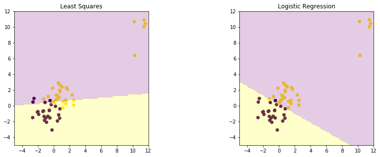
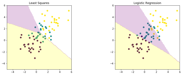
The Least squares fails on many aspects:

• lacks roubustness: highly sensitive to outliers

• gives poor classification: assign small region to the middle cluster

The failure of least squares should not surprise us when we recall that it corresponds to maximum likelihood under the assumption of a Gaussian conditional distribution, whereas binary target vectors clearly have a distribution that is far from Gaussian.

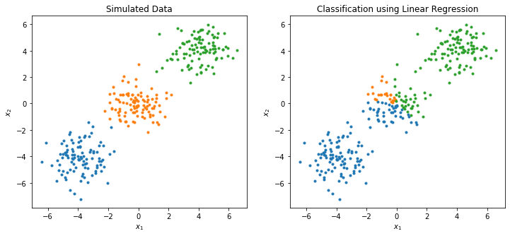
There is a serious problem with the least squares approach when \(K \ge 3\) where classes can be masked by others. Consider an extreme situation with simulated dataset as follows.

The middle class is mostly masked (dominated) by other two classes as many points of the middle class are assigned colors of other two classes.

size = 100
np.random.seed(123)
x0 = np.random.multivariate_normal([-4, -4], np.eye(2), size)
x1 = np.random.multivariate_normal([ 0,  0], np.eye(2), size)
x2 = np.random.multivariate_normal([ 4,  4], np.eye(2), size)
x = np.concatenate((x0, x1, x2))
x_tilde = np.hstack((np.ones((size*3, 1)), x))
t1, t2, t3 = np.eye(3)
t = np.vstack((np.tile(t1, (size, 1)),
               np.tile(t2, (size, 1)),
               np.tile(t3, (size, 1))))

reg = LinearRegression().fit(x, t)
y = reg.predict(x)
t_pred = y.argmax(axis=1)

from sklearn.preprocessing import PolynomialFeatures
from sklearn.pipeline import Pipeline
polyreg = Pipeline([('poly', PolynomialFeatures(degree=2)),
                  ('linear', LinearRegression())])
poly_y = polyreg.fit(x, t).predict(x)

plt.figure(figsize=(12, 5))
plt.subplot(1, 2, 1)
plt.plot(x0[:,0], x0[:,1], 'o', color='C0', markersize=3)
plt.plot(x1[:,0], x1[:,1], 'o', color='C1', markersize=3)
plt.plot(x2[:,0], x2[:,1], 'o', color='C2', markersize=3)
plt.xlabel('$x_1$')
plt.ylabel('$x_2$')
plt.title('Simulated Data')

plt.subplot(1, 2, 2)
plt.plot(x[t_pred == 0][:,0], x[t_pred == 0][:,1], 'o', color='C0', markersize=3)
plt.plot(x[t_pred == 1][:,0], x[t_pred == 1][:,1], 'o', color='C1', markersize=3)
plt.plot(x[t_pred == 2][:,0], x[t_pred == 2][:,1], 'o', color='C2', markersize=3)
plt.xlabel('$x_1$')
plt.ylabel('$x_2$')
plt.title('Classification using Linear Regression')

plt.show()
toggle()

show code

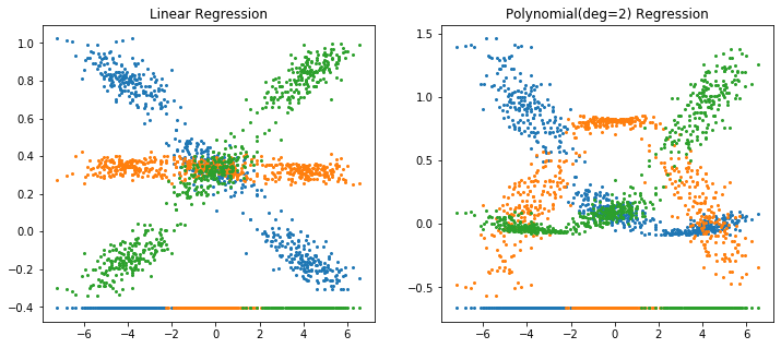
For each simulated point \((x_1, x_2)\), we have its \(y\) (or \(\hat{y}\)) value based on linear (or degree 2 polynomial) regression equation, where \(y\) (or \(\hat{y}\)) has three components corresponding to three probabilities for each class.

The plot(x, y[:, 0], 'o', color='C0', markersize=2) function plots two points \((x_1, y_0)\) and \((x_2, y_0)\) where \(y_0\) is the probability that this point is in the first class.

The classified class is defined as

\begin{align*} k^* = \text{argmax}_k \{y_k(\mathbf{x}): k = 1,\ldots,K\} \end{align*}

or t_pred = reg.predict(x).argmax(axis=1).

Because of this argmax operator, the middle class cannot be identified in linear regression model, but can be identified in a polynomial regression model.

fig = plt.figure(1, figsize=(12, 5))
ax1 = fig.add_subplot(1, 2, 1)
ax1.plot(x, y[:, 0], 'o', color='C0', markersize=2)
ax1.plot(x, y[:, 1], 'o', color='C1', markersize=2)
ax1.plot(x, y[:, 2], 'o', color='C2', markersize=2)
y_floor, _ = ax1.get_ylim()
ax1.plot(x0, [y_floor]*size, 'o', color='C0', markersize=2)
ax1.plot(x1, [y_floor]*size, 'o', color='C1', markersize=2)
ax1.plot(x2, [y_floor]*size, 'o', color='C2', markersize=2)
ax1.set_title('Linear Regression')

ax2 = fig.add_subplot(1, 2, 2)
ax2.plot(x, poly_y[:, 0], 'o', color='C0', markersize=2)
ax2.plot(x, poly_y[:, 1], 'o', color='C1', markersize=2)
ax2.plot(x, poly_y[:, 2], 'o', color='C2', markersize=2)
y_floor, _ = ax2.get_ylim()
ax2.plot(x0, [y_floor]*size, 'o', color='C0', markersize=2)
ax2.plot(x1, [y_floor]*size, 'o', color='C1', markersize=2)
ax2.plot(x2, [y_floor]*size, 'o', color='C2', markersize=2)
ax2.set_title('Polynomial(deg=2) Regression')
plt.show()
toggle()

show code

Linear Discriminant Analysis

Linear Discriminant Analysis (LDA) is most commonly used as dimensionality reduction technique in the pre-processing step for pattern-classification and machine learning applications. The goal is to project a dataset onto a lower-dimensional space with good class-separability in order avoid overfitting (“curse of dimensionality”) and also reduce computational costs.

For optimal classification, we need to know the class posteriors \(p(\mathcal{C}_k | \mathbf{x})\) of our observation \(\mathbf{x}\):

\begin{align*} p(\mathcal{C}_k | \mathbf{x}) = \frac{p(\mathbf{x}|\mathcal{C}_k)p(\mathcal{C}_k)}{p(\mathbf{x})} = \frac{p(\mathbf{x}|\mathcal{C}_k)p(\mathcal{C}_k)}{\sum_{j}p(\mathbf{x}|\mathcal{C}_j)p(\mathcal{C}_j)} \end{align*}

Assume class-conditional densities are Gaussian with common covariance matrix \(\Sigma\).

\begin{align} p(\mathbf{x}|\mathcal{C}_k) = \frac{1}{(2\pi)^{D/2}} \frac{1}{\lvert \Sigma \rvert ^{1/2}} \exp \left( -\frac{1}{2} (\mathbf{x} - \mathbf{\mu}_k)^\intercal \Sigma^{-1} (\mathbf{x} - \mathbf{\mu}_k) \right) \nonumber \end{align}

If \(p(\mathbf{x}|\mathcal{C}_k)\) has its own covariance matrix \(\Sigma_k\), then we will obtain \(y_k(\mathbf{x})\) as a quadratic discriminant function of \(\mathbf{x}\), giving rise to a quadratic discriminant analysis.

When comparing two classes \(k\), \(\ell\) by \(p(\mathcal{C}_k | \mathbf{x}) - p(\mathcal{C}_\ell | \mathbf{x})\), it is sufficient to consider

\begin{align} \ln p(\mathcal{C}_k| \mathbf{x}) - \ln p(\mathcal{C}_\ell | \mathbf{x}) &= \ln \frac{p(\mathcal{C}_k | \mathbf{x})}{p(\mathcal{C}_\ell | \mathbf{x})} = \ln \frac{p(\mathbf{x}|\mathcal{C}_k)p(\mathcal{C}_k)}{p(\mathbf{x}|\mathcal{C}_\ell)p(\mathcal{C}_\ell)} \nonumber \\ & = \mathbf{x}^\intercal \Sigma^{-1} (\mu_k - \mu_\ell) - \frac{1}{2} (\mu_k+\mu_\ell)^\intercal \Sigma^{-1} (\mu_k - \mu_\ell) + \ln \frac{p(\mathcal{C}_k)}{p(\mathcal{C}_\ell)} \tag{LDA} \\ & \equiv \ln \frac{y_k(\mathbf{x})}{y_\ell(\mathbf{x})} \nonumber \end{align}

The discriminant function \begin{align*} y_k(\mathbf{x}) = \ln p(\mathbf{x}|\mathcal{C}_k)p(\mathcal{C}_k) &= \mathbf{w}^\intercal_k \mathbf{x} + w_{k0} \text{ where}\\ \mathbf{w}_k &= \Sigma^{-1} \mu_k \\ w_{k0} &= - \frac{1}{2} \mu^\intercal_k \Sigma^{-1} \mu_k + \ln p(\mathcal{C}_k) \end{align*}

The parameters of the Gaussian distributions are estimated through training data

• \(p(\mathcal{C}_k) = n_k / n\) where \(n_k\) is the number of class-\(k\) observations

• \(\mu_k = \sum_{j \in \mathcal{C}_k} \mathbf{x}_j / n_k\)

• \(\Sigma = 1/n \sum_{k=1}^{K} \sum_{j \in \mathcal{C}_k} (\mathbf{x}_j - \mu_k)^\intercal (\mathbf{x}_j - \mu_k)\)

Fisher’s Linear Discriminant

Fisher derived LDA via a route without referring to Gaussian distributions.

Fisher’s idea is to maximize a function that

• give a large separation between the projected class means

• give a small variance within each class

thereby minimizing the class overlap.

Consider a two-class problem with \(n_1\) points of class \(\mathcal{C}_1\) and \(n_2\) points of class \(\mathcal{C}_2\)

• We need reduce \(p\)-dimension \(\mathbf{x}\) to one dimension using \(y = \mathbf{w}^\intercal \mathbf{x}\)

• We choose \(\mathbf{w}\) to maximize \(\mathbf{w}^\intercal(\mathbf{m}_1-\mathbf{m}_2) \equiv m_1-m_2\), with scaler \(\sum_{i} w^2_i=1\).

where the mean vectors of two classes

\begin{align} \mathbf{m}_1 = \frac{1}{n_1} \sum_{i \in \mathcal{C}_1} \mathbf{x}_i \text{ and } \mathbf{m}_2 = \frac{1}{n_2} \sum_{i \in \mathcal{C}_2} \mathbf{x}_i \nonumber \end{align}

We can get

\begin{align} \mathbf{w} \propto S^{-1}_W(\mathbf{m}_2-\mathbf{m}_1) \nonumber \end{align}

where \(S_W\) is the total within-class covariance matrix. Note \(S^{-1}_W\) is equivalent to \(\Sigma^{-1}\) in (LDA). Hence, Fisher’s method gives the same discriminant function as in (LDA).

hide_comment()

show comment

Fisher’s method is to maximize

\begin{align} J(\mathbf{w}) &= \frac{(m_1 - m_2)^2}{\sum_{k=1}^{2}\sum_{i \in \mathcal{C}_k} (y_i-m_k)^2} = \frac{\text{between class variance}}{\text{within class variance}} \nonumber \\ &= \frac{\mathbf{w}^\intercal (\mathbf{m}_2-\mathbf{m}_1) \bigg(\mathbf{w}^\intercal(\mathbf{m}_2-\mathbf{m}_1)\bigg)^\intercal}{\sum_{k=1}^{2} \sum_{i \in \mathcal{C}_k} \mathbf{w}^\intercal(\mathbf{x}_i - \mathbf{m}_1) \bigg(\mathbf{w}^\intercal(\mathbf{x}_i - \mathbf{m}_1)\bigg)^\intercal} \nonumber \\ &= \frac{\mathbf{w}^\intercal (\mathbf{m}_2-\mathbf{m}_1)(\mathbf{m}_2-\mathbf{m}_1)^\intercal \mathbf{w}}{\mathbf{w}^\intercal \sum_{k=1}^{2} \sum_{i \in \mathcal{C}_k} (\mathbf{x}_i - \mathbf{m}_k)(\mathbf{x}_i - \mathbf{m}_k)^\intercal \mathbf{w}} \nonumber \\ &\equiv \frac{\mathbf{w}^\intercal \mathbf{S}_B \mathbf{w}}{\mathbf{w}^\intercal \mathbf{S}_W \mathbf{w}} \nonumber \end{align}

\begin{align} J^\prime(\mathbf{w}) &= 0 \Rightarrow \left(\mathbf{w}^\intercal \mathbf{S}_W \mathbf{w}\right) \mathbf{S}_B \mathbf{w} = \left(\mathbf{w}^\intercal \mathbf{S}_B \mathbf{w}\right) \mathbf{S}_W \mathbf{w} \Rightarrow \mathbf{w} \propto S^{-1}_W(\mathbf{m}_2-\mathbf{m}_1) \nonumber \end{align}

For general \(K\), Fisher’s method is to maximize so called Rayleigh quotient

\begin{align} \max_{\mathbf{w}} J(\mathbf{w}) = \frac{\mathbf{w}^\intercal \mathbf{S}_B \mathbf{w}}{\mathbf{w}^\intercal \mathbf{S}_W \mathbf{w}} = \frac{\text{between class variance}}{\text{within class variance}} \nonumber \end{align}

where \begin{align*} S_B &= \sum_{k=1}^{K} n_{k} (\mathbf{m}_k - \mathbf{m}) (\mathbf{m}_k - \mathbf{m})^\intercal \\ S_W &= \sum_{k=1}^{K} S_k \text{ with } S_k = \sum_{i \in \mathcal{C}_k} (\mathbf{x}_i - \mathbf{m}_k) (\mathbf{x}_i - \mathbf{m}_k)^\intercal \end{align*}

\begin{align*} \mathbf{m}_k &= \frac{1}{n_k} \sum_{i \in \mathcal{C}_k} \mathbf{x}_i \\ \mathbf{m} &= \frac{1}{n} \sum_{i=1}^{n} \mathbf{x}_i = \frac{1}{n} \sum_{k=1}^{K} n_k \mathbf{m}_k \end{align*}

and \(n_k\) is the sample size of the class \(k\).

Because \(J(\mathbf{w})\) is invariant w.r.t. rescaling of \(\mathbf{w} \leftarrow \alpha \mathbf{w}\), so that we can choose \(\alpha\) as to have a unit denominator \(\mathbf{w}^\intercal S_W \mathbf{w} = 1\) (since it is a scalar). Thus

\begin{align*} \max_{\mathbf{w}}~ J(\mathbf{w}) = \min_{\mathbf{w}} - \mathbf{w}^\intercal S_B \mathbf{w} ~\text{ s.t. } \mathbf{w}^\intercal S_W \mathbf{w} = 1 \end{align*}

Let \(\mathbf{w}^\ast = S_W^{1/2} \mathbf{w}\) and \(S^*_B = (S_W^{-1/2})^\intercal S_B S_W^{-1/2}\), we have

\begin{align*} \min_{\mathbf{w}^*}~ -(\mathbf{w}^*)^\intercal S^*_B \mathbf{w}^* ~\text{ s.t. } (\mathbf{w}^*)^\intercal \mathbf{w}^* = 1 \end{align*}

Note that let \(M\) be the \(K \times p\) matrix of centroids \(\mu_k\). Then

\begin{align*} S_B &= M^\intercal M \\ S^*_B &= (M S_W^{-1/2})^\intercal (M S_W^{-1/2}) \end{align*}

The Lagrangien is

\begin{align*} L = -(\mathbf{w}^{*})^{\intercal}S_B^{*}\mathbf{w}^{*} + \lambda[(\mathbf{w}^{*})^{\intercal}\mathbf{w}^{*}-1] \end{align*}

Its derivative gives

\begin{align*} S_B^{*}\mathbf{w}^{*}=\lambda \mathbf{w}^{*} \end{align*}

The optimization becomes an eigendecomposition problem.

The relationship between LDA and linear regression

When \(K=2\), there is a simple correspondence between LDA and linear regression:

we adopt a different target coding scheme that

• \(t_i =n/n_1\) if the input \(\mathbf{x}_i\) is in class \(\mathcal{C}_1\) (the value approximates the reciprocal of the prior probability for class \(\mathcal{C}_1\)) and;

• \(t_i = -n/n_2\) if the input \(\mathbf{x}_i\) is in class \(\mathcal{C}_2\),

where \(n\) is the total number observations and \(n_k\) (\(k=1, 2\)) is the number observations in class \(k\).

Minimizing the sum of squares error function

\begin{align} \frac{1}{2} \sum_{i=1}^{n} \left(\mathbf{w}^\intercal \mathbf{x}_i + w_0 - t_i \right)^2 \text{ gives } \mathbf{w} \propto S^{-1}_W(\mathbf{m}_2-\mathbf{m}_1) \nonumber \end{align}

\(\blacksquare\)

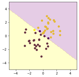
The code demonstrate the implementation of Fisher’s method for 2-class data:

x_train, t_train = train_data['2-class']
x1_test, x2_test = np.meshgrid(np.linspace(-5, 5, 100), np.linspace(-5, 5, 100))
x_test = np.array([x1_test, x2_test]).reshape(2, -1).T

X0 = x_train[t_train == 0]
X1 = x_train[t_train == 1]
m0 = np.mean(X0, axis=0)
m1 = np.mean(X1, axis=0)
cov_inclass = (X0 - m0).T @ (X0 - m0) + (X1 - m1).T @ (X1 - m1)
w = np.linalg.solve(cov_inclass, m1 - m0)
w /= np.linalg.norm(w).clip(min=1e-10)

mu0 = np.mean(X0 @ w, axis=0)
mu1 = np.mean(X1 @ w, axis=0)
var0 = np.var(X0 @ w, axis=0)
var1 = np.var(X1 @ w, axis=0)
a = var1 - var0
b = var0 * mu1 - var1 * mu0
c = var1 * mu0 ** 2 - var0 * mu1 ** 2 - var1 * var0 * np.log(var1 / var0)
threshold = (np.sqrt(b ** 2 - a * c) - b) / a

t = (x_test @ w > threshold).astype(np.int)

plt.scatter(x_train[:, 0], x_train[:, 1], c=t_train)
plt.contourf(x1_test, x2_test, t.reshape(100, 100), alpha=0.2, levels=np.linspace(0, 1, 3),
             cmap=matplotlib.colors.ListedColormap(['yellow','green','purple']))
plt.xlim(-5, 5)
plt.ylim(-5, 5)
plt.gca().set_aspect('equal', adjustable='box')
plt.show()

toggle()

show code

LDA: Iris Data

Consider the famous “Iris” dataset which contains measurements for 150 iris flowers from three different species.

The three classes (\(K=3\)) in the Iris dataset:

• Iris-setosa (n=50)

• Iris-versicolor (n=50)

• Iris-virginica (n=50)

The four features (\(p=4\)) of the Iris dataset:

• sepal length in cm

• sepal width in cm

• petal length in cm

• petal width in cm

feature_dict = {i:label for i,label in zip(
                range(4),
                  ('sepal length in cm',
                  'sepal width in cm',
                  'petal length in cm',
                  'petal width in cm', ))}
df = pd.read_csv(
    'https://raw.githubusercontent.com/ming-zhao/Optimization-and-Learning/master/data/iris.data',
    header=None, sep=',')
df.columns = [l for i,l in sorted(feature_dict.items())] + ['class label']
df.dropna(how="all", inplace=True) # to drop the empty line at file-end
df.tail()
toggle()

show code

We define

\begin{align} \pmb X = \begin{bmatrix} x_{1_{\text{sepal length}}} & x_{1_{\text{sepal width}}} & x_{1_{\text{petal length}}} & x_{1_{\text{petal width}}}\\ x_{2_{\text{sepal length}}} & x_{2_{\text{sepal width}}} & x_{2_{\text{petal length}}} & x_{2_{\text{petal width}}}\\ ... \\ x_{150_{\text{sepal length}}} & x_{150_{\text{sepal width}}} & x_{150_{\text{petal length}}} & x_{150_{\text{petal width}}}\\ \end{bmatrix}, ~~ \pmb y = \begin{bmatrix} \omega_{\text{setosa}}\\ \omega_{\text{setosa}}\\ ... \\ \omega_{\text{virginica}}\end{bmatrix} \nonumber \end{align}

We use the LabelEncode from the scikit-learn library to convert the class labels into numbers: 1, 2, and 3.

from sklearn.preprocessing import LabelEncoder
X = df[df.columns[:-1]].values
y = df['class label'].values

enc = LabelEncoder()
label_encoder = enc.fit(y)
y = label_encoder.transform(y) + 1

label_dict = {1: 'Setosa', 2: 'Versicolor', 3:'Virginica'}
toggle()

show code

\begin{align*} \pmb y = \begin{bmatrix}{\text{setosa}}\\ {\text{setosa}}\\ ... \\ {\text{virginica}}\end{bmatrix} \quad \Rightarrow \begin{bmatrix} {\text{1}}\\ {\text{1}}\\ ... \\ {\text{3}}\end{bmatrix} \end{align*}

Histograms and feature selection

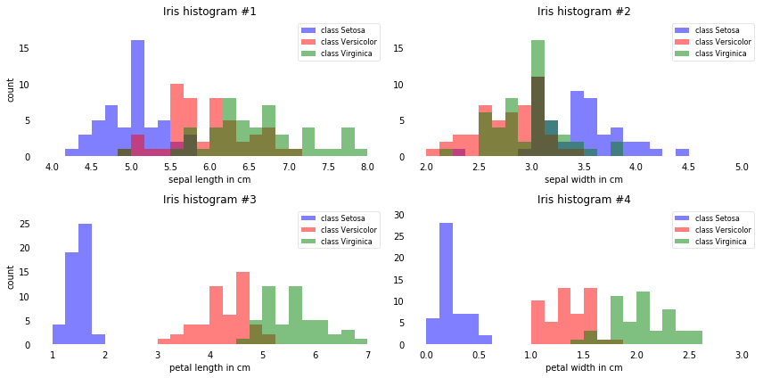
To get a rough idea how the samples of three classes are distributed, let us visualize the distributions of the four different features in 1-dimensional histograms.

fig, axes = plt.subplots(nrows=2, ncols=2, figsize=(12,6))

for ax,cnt in zip(axes.ravel(), range(4)):

    # set bin sizes
    min_b = np.floor(np.min(X[:,cnt]))
    max_b = np.ceil(np.max(X[:,cnt]))
    bins = np.linspace(min_b, max_b, 25)

    # plottling the histograms
    for lab,col in zip(range(1,4), ('blue', 'red', 'green')):
        ax.hist(X[y==lab, cnt],
                   color=col,
                   label='class %s' %label_dict[lab],
                   bins=bins,
                   alpha=0.5,)
    ylims = ax.get_ylim()

    # plot annotation
    leg = ax.legend(loc='upper right', fancybox=True, fontsize=8)
    leg.get_frame().set_alpha(0.5)
    ax.set_ylim([0, max(ylims)+2])
    ax.set_xlabel(feature_dict[cnt])
    ax.set_title('Iris histogram #%s' %str(cnt+1))

    # hide axis ticks
    ax.tick_params(axis="both", which="both", bottom=False, top=False,
            labelbottom=True, left=False, right=False, labelleft=True)

    # remove axis spines
    ax.spines["top"].set_visible(False)
    ax.spines["right"].set_visible(False)
    ax.spines["bottom"].set_visible(False)
    ax.spines["left"].set_visible(False)

axes[0][0].set_ylabel('count')
axes[1][0].set_ylabel('count')

fig.tight_layout()

plt.show()
toggle()

show code

From just looking at these simple graphical representations of the features, we can already tell that the petal lengths and widths (histogram #3 and #4) are likely better suited as potential features two separate between the three flower classes.

In practice, instead of reducing the dimensionality via a projection (here: LDA), a good alternative would be a feature selection technique. For low-dimensional datasets like Iris, a glance at those histograms would already be very informative. Another simple, but very useful technique would be to use feature selection algorithms.

LDA assumes normal distributed data, features that are statistically independent, and identical covariance matrices for every class. However, LDA can work reasonably well if those assumptions are violated.

In practice, LDA for dimensionality reduction would be just another preprocessing step for a typical machine learning or pattern classification task.

Computing Mean Vectors

In this first step, we will start off with a simple computation of the mean vectors \(\mathbf{m}_i\), \(i=1,2,3\) of the 3 different flower classes:

\begin{align*} \mathbf{m}_i = \begin{bmatrix} \mu_{\omega_i (\text{sepal length)}}\\ \mu_{\omega_i (\text{sepal width})}\\ \mu_{\omega_i (\text{petal length)}}\\ \mu_{\omega_i (\text{petal width})}\\ \end{bmatrix} \; , \quad \text{with} \quad i = 1,2,3 \end{align*}

np.set_printoptions(precision=4)

mean_vectors = []
for cl in range(1,4):
    mean_vectors.append(np.mean(X[y==cl], axis=0))
    print('Mean Vector class %s: %s\n' %(cl, mean_vectors[cl-1]))

toggle()

Mean Vector class 1: [5.006 3.418 1.464 0.244]

Mean Vector class 2: [5.936 2.77  4.26  1.326]

Mean Vector class 3: [6.588 2.974 5.552 2.026]

show code

Computing the Scatter Matrices

Now, we will compute the two \(4 \times 4\) \((p \times p)\)-dimensional matrices: The within-class and the between-class scatter matrix.

Within-class scatter matrix \begin{align*} S_W = \sum_{k=1}^{K} S_k \end{align*}

where \begin{align*} S_k &= \sum_{i \in \mathcal{C}_k} (\mathbf{x}_i - \mathbf{m}_k) (\mathbf{x}_i - \mathbf{m}_k)^\intercal \\ \mathbf{m}_k &= \frac{1}{n_k} \sum_{i \in \mathcal{C}_k} \mathbf{x}_i \end{align*}

and \(n_k\) is the sample size of the class \(k\).

S_W = np.zeros((4,4))
for cl,mv in zip(range(1,4), mean_vectors):
    class_sc_mat = np.zeros((4,4))                  # scatter matrix for every class
    for row in X[y == cl]:
        row, mv = row.reshape(4,1), mv.reshape(4,1) # make column vectors
        class_sc_mat += (row-mv).dot((row-mv).T)
    S_W += class_sc_mat                             # sum class scatter matrices
print('within-class Scatter Matrix:\n', S_W)

toggle()

within-class Scatter Matrix:
 [[38.9562 13.683  24.614   5.6556]
 [13.683  17.035   8.12    4.9132]
 [24.614   8.12   27.22    6.2536]
 [ 5.6556  4.9132  6.2536  6.1756]]

show code

The total variance matrix \begin{align*} S_T = \sum_{i=1}^{n} (\mathbf{x}_i - \mathbf{m}) (\mathbf{x}_i - \mathbf{m})^\intercal \end{align*}

where \(\mathbf{m}\) is the mean of total data set

\begin{align*} \mathbf{m} = \frac{1}{n} \sum_{i=1}^{n} \mathbf{x}_i = \frac{1}{n} \sum_{k=1}^{K} n_k \mathbf{m}_k \end{align*}

\begin{align*} S_T = S_W + S_B \end{align*}

where \(S_B\) is between-class scatter matrix

\begin{align*} S_B = \sum_{k=1}^{K} N_{k} (\mathbf{m}_k - \mathbf{m}) (\mathbf{m}_k - \mathbf{m})^\intercal \end{align*}

overall_mean = np.mean(X, axis=0)

S_B = np.zeros((4,4))
for i,mean_vec in enumerate(mean_vectors):
    n = X[y==i+1,:].shape[0]
    mean_vec = mean_vec.reshape(4,1) # make column vector
    overall_mean = overall_mean.reshape(4,1) # make column vector
    S_B += n * (mean_vec - overall_mean).dot((mean_vec - overall_mean).T)

print('between-class Scatter Matrix:\n', S_B)
toggle()

between-class Scatter Matrix:
 [[ 63.2121 -19.534  165.1647  71.3631]
 [-19.534   10.9776 -56.0552 -22.4924]
 [165.1647 -56.0552 436.6437 186.9081]
 [ 71.3631 -22.4924 186.9081  80.6041]]

show code

Solving the Generalized Eigenvalue Problem

Next, we will solve the generalized eigenvalue problem for the matrix \(S^{-1}_W S_B\) to obtain the linear discriminants where

\begin{align*} (S^{-1}_W S_B) v = \lambda v \end{align*}

• \(\lambda\): eigenvalue

• \(v\): eigenvector

eig_vals, eig_vecs = np.linalg.eig(np.linalg.inv(S_W).dot(S_B))

for i in range(len(eig_vals)):
    eigvec_sc = eig_vecs[:,i].reshape(4,1)
    print('\nEigenvector {}: \n{}'.format(i+1, eigvec_sc.real))
    print('Eigenvalue {:}: {:.2e}'.format(i+1, eig_vals[i].real))

toggle()

Eigenvector 1:
[[-0.2049]
 [-0.3871]
 [ 0.5465]
 [ 0.7138]]
Eigenvalue 1: 3.23e+01

Eigenvector 2:
[[-0.009 ]
 [-0.589 ]
 [ 0.2543]
 [-0.767 ]]
Eigenvalue 2: 2.78e-01

Eigenvector 3:
[[-0.8844]
 [ 0.2854]
 [ 0.258 ]
 [ 0.2643]]
Eigenvalue 3: 3.42e-15

Eigenvector 4:
[[-0.2234]
 [-0.2523]
 [-0.326 ]
 [ 0.8833]]
Eigenvalue 4: 1.15e-14

show code

Recall from our linear algebra, both eigenvectors and eigenvalues are providing us with information about the distortion of a linear transformation: The eigenvectors are basically the direction of this distortion, and the eigenvalues are the scaling factor for the eigenvectors that describing the magnitude of the distortion.

If we are performing the LDA for dimensionality reduction, the eigenvectors are important since they will form the new axes of our new feature subspace; the associated eigenvalues are of particular interest since they will tell us how “informative” the new “axes” are.

Checking the eigenvector-eigenvalue calculation

for i in range(len(eig_vals)):
    eigv = eig_vecs[:,i].reshape(4,1)
    np.testing.assert_array_almost_equal(np.linalg.inv(S_W).dot(S_B).dot(eigv),
                                         eig_vals[i] * eigv,
                                         decimal=6, err_msg='', verbose=True)
# print('ok')
toggle()

show code

Constructing the New Feature Subspace

We are interested in

• projecting the data into a subspace that improves the class separability,

• reducing the dimensionality of our feature space, where the eigenvectors will form the axes of this new feature subspace.

So, in order to decide which eigenvector(s) we want to drop for our lower-dimensional subspace, we have to take a look at the corresponding eigenvalues of the eigenvectors (eigenvectors all have all the same unit length 1).

Roughly speaking, the eigenvectors with the lowest eigenvalues bear the least information about the distribution of the data, and those are the ones we want to drop.

The common approach is to rank the eigenvectors from highest to lowest corresponding eigenvalue and choose the top \(C\) eigenvectors.

# Make a list of (eigenvalue, eigenvector) tuples
eig_pairs = [(np.abs(eig_vals[i]), eig_vecs[:,i]) for i in range(len(eig_vals))]

# Sort the (eigenvalue, eigenvector) tuples from high to low
eig_pairs = sorted(eig_pairs, key=lambda k: k[0], reverse=True)

# Visually confirm that the list is correctly sorted by decreasing eigenvalues

print('Eigenvalues in decreasing order:\n')
for i in eig_pairs:
    print(i[0])
toggle()

Eigenvalues in decreasing order:

32.27195779972981
0.27756686384003953
1.1483362279322388e-14
3.422458920849769e-15

show code

In fact, these two last eigenvalues should be exactly zero. They are not because of floating-point imprecision.

In LDA, the number of linear discriminants is at most \(K-1\) where \(K\) is the number of class labels, since the in-between scatter matrix \(S_B\) is the sum of \(K\) matrices with rank 1 or less.

Now, let’s express the “explained variance” as percentage:

print('Variance explained:\n')
eigv_sum = sum(eig_vals)
for i,j in enumerate(eig_pairs):
    print('eigenvalue {0:}: {1:.2%}'.format(i+1, (j[0]/eigv_sum).real))

toggle()

Variance explained:

eigenvalue 1: 99.15%
eigenvalue 2: 0.85%
eigenvalue 3: 0.00%
eigenvalue 4: 0.00%

show code

The first eigenpair is by far the most informative one, and we won’t loose much information if we would form a 1D-feature spaced based on this eigenpair.

Now choose \(K\) eigenvectors with the largest eigenvalues

After sorting the eigenpairs by decreasing eigenvalues, it is now time to construct our \(p \times C\)-dimensional eigenvector matrix \(W\) (here \(4 \times 2\): based on the 2 most informative eigenpairs) and thereby reducing the initial 4-dimensional feature space into a 2-dimensional feature subspace.

W = np.hstack((eig_pairs[0][1].reshape(4,1), eig_pairs[1][1].reshape(4,1)))
print('Matrix W:\n', W.real)
toggle()

Matrix W:
 [[-0.2049 -0.009 ]
 [-0.3871 -0.589 ]
 [ 0.5465  0.2543]
 [ 0.7138 -0.767 ]]

show code

Transforming the samples

We use \(W\) to transform our samples onto the new subspace via the equation

\begin{align*} Y = X_{n \times p} W_{p \times C} \end{align*}

X_lda = X.dot(W)
assert X_lda.shape == (150,2), "The matrix is not 150x2 dimensional."

from matplotlib import pyplot as plt

def plot_step_lda():

    ax = plt.subplot(111)
    for label,marker,color in zip(
        range(1,4),('^', 's', 'o'),('blue', 'red', 'green')):

        plt.scatter(x=X_lda[:,0].real[y == label],
                y=X_lda[:,1].real[y == label],
                marker=marker,
                color=color,
                alpha=0.5,
                label=label_dict[label]
                )

    plt.xlabel('LD1')
    plt.ylabel('LD2')

    leg = plt.legend(loc='upper right', fancybox=True)
    leg.get_frame().set_alpha(0.5)
    plt.title('LDA: Iris projection onto the first 2 linear discriminants')

    # hide axis ticks
    plt.tick_params(axis="both", which="both", bottom=False, top=False,
            labelbottom=True, left=False, right=False, labelleft=True)

    # remove axis spines
    ax.spines["top"].set_visible(False)
    ax.spines["right"].set_visible(False)
    ax.spines["bottom"].set_visible(False)
    ax.spines["left"].set_visible(False)

    plt.grid()
    plt.tight_layout
    plt.show()

plot_step_lda()
toggle()

show code

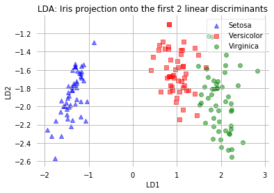
The scatter plot above represents our new feature subspace that we constructed via LDA. We can see that the first linear discriminant “LD1” separates the classes quite nicely. However, the second discriminant, “LD2”, does not add much valuable information, which we’ve already concluded when we looked at the ranked eigenvalues is step 4.

PCA vs LDA

Both Linear Discriminant Analysis (LDA) and Principal Component Analysis (PCA) are linear transformation techniques that are commonly used for dimensionality reduction.

• PCA can be described as an “unsupervised” algorithm, since it “ignores” class labels and its goal is to find the directions (the so-called principal components) that maximize the variance in a dataset.

• LDA is “supervised” and computes the directions (“linear discriminants”) that will represent the axes that that maximize the separation between multiple classes.

Although it might sound intuitive that LDA is superior to PCA for a multi-class classification task where the class labels are known, this might not always the case. For example, comparisons between classification accuracies for image recognition after using PCA or LDA show that PCA tends to outperform LDA if the number of samples per class is relatively small (PCA vs. LDA, A.M. Martinez et al., 2001).

In practice, often a LDA follows a PCA for dimensionality reduction (PCA can be performed before LDA to regularize the problem and avoid over-fitting).

There is a more convenient way to achieve the same via the LDA classifier (or PCA) implemented in the scikit-learn.

from sklearn.decomposition import PCA as sklearnPCA
from sklearn.discriminant_analysis import LinearDiscriminantAnalysis as LDA

sklearn_lda = LDA(n_components=2)
X_lda_sklearn = sklearn_lda.fit_transform(X, y)
def plot_scikit_lda(X, title):

    ax = plt.subplot(111)
    for label,marker,color in zip(
        range(1,4),('^', 's', 'o'),('blue', 'red', 'green')):

        plt.scatter(x=X[:,0][y == label],
                    y=X[:,1][y == label] * -1, # flip the figure
                    marker=marker,
                    color=color,
                    alpha=0.5,
                    label=label_dict[label])

    plt.xlabel('LD1')
    plt.ylabel('LD2')

    leg = plt.legend(loc='upper right', fancybox=True)
    leg.get_frame().set_alpha(0.5)
    plt.title(title)

    # hide axis ticks
    plt.tick_params(axis="both", which="both", bottom=False, top=False,
            labelbottom=True, left=False, right=False, labelleft=True)

    # remove axis spines
    ax.spines["top"].set_visible(False)
    ax.spines["right"].set_visible(False)
    ax.spines["bottom"].set_visible(False)
    ax.spines["left"].set_visible(False)

    plt.grid()
    plt.tight_layout
    plt.show()

sklearn_pca = sklearnPCA(n_components=2)
X_pca = sklearn_pca.fit_transform(X)
def plot_pca():

    ax = plt.subplot(111)

    for label,marker,color in zip(
        range(1,4),('^', 's', 'o'),('blue', 'red', 'green')):

        plt.scatter(x=X_pca[:,0][y == label],
                y=X_pca[:,1][y == label],
                marker=marker,
                color=color,
                alpha=0.5,
                label=label_dict[label]
                )

    plt.xlabel('PC1')
    plt.ylabel('PC2')

    leg = plt.legend(loc='upper right', fancybox=True)
    leg.get_frame().set_alpha(0.5)
    plt.title('PCA: Iris projection onto the first 2 principal components')

    # hide axis ticks
    plt.tick_params(axis="both", which="both", bottom=False, top=False,
            labelbottom=True, left=False, right=False, labelleft=True)

    # remove axis spines
    ax.spines["top"].set_visible(False)
    ax.spines["right"].set_visible(False)
    ax.spines["bottom"].set_visible(False)
    ax.spines["left"].set_visible(False)

    plt.tight_layout
    plt.grid()

    plt.show()

toggle()

show code

plot_scikit_lda(X_lda_sklearn, title='Default LDA via scikit-learn')
plot_pca()

toggle()

show code

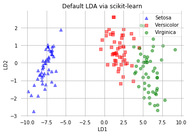
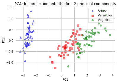
The two plots above nicely confirm what we have discussed before: Where the PCA accounts for the most variance in the whole dataset, the LDA gives us the axes that account for the most variance between the individual classes.

Generative Models

We consider

• the class-conditional density \(p(\mathbf{x}|\mathcal{C}_k)\) with a specified parametric functional form, and

• the class prior \(p(\mathcal{C}_k)\)

• then compute posterior probability \(p(\mathcal{C}_k|\mathbf{x})\) through Bayes’ theorem.

The indirect (comparing to model \(p(\mathcal{C}_k|\mathbf{x})\) directly) is an example of generative modeling, because we can generate synthetic data by drawing values of \(\mathbf{x}\) from \(p(\mathbf{x})\).

Continuous Features

Consider \(K=2\), we have \begin{align} p(\mathcal{C}_1 | \mathbf{x}) = \frac{p(\mathbf{x}|\mathcal{C}_1)p(\mathcal{C}_1)}{p(\mathbf{x}|\mathcal{C}_1)p(\mathcal{C}_1) + p(\mathbf{x}|\mathcal{C}_2)p(\mathcal{C}_2)} = \frac{1}{1+\exp(-a)} = \sigma(a) \nonumber \end{align}

with \begin{align} a = \ln \frac{p(\mathbf{x}|\mathcal{C}_1)p(\mathcal{C}_1)}{p(\mathbf{x}|\mathcal{C}_2)p(\mathcal{C}_2)} \triangleq \mathbf{w}^\intercal \mathbf{x} \label{eqn_act} \end{align}

where \(\sigma(\cdot)\) is the logistic sigmoid function.

For general \(K > 2\),

\begin{align*} p(\mathcal{C}_k | \mathbf{x}) &= \frac{p(\mathbf{x}|\mathcal{C}_k)p(\mathcal{C}_k)}{\sum_{j}p(\mathbf{x}|\mathcal{C}_j)p(\mathcal{C}_j)} \\ &= \frac{\exp(a_k)}{\sum_{j}\exp(a_j)} = \text{softmax}_k (a) \end{align*}

where the activate function

\begin{align*} a_k = \ln p(\mathbf{x}|\mathcal{C}_k)p(\mathcal{C}_k) \end{align*}

and softmax function represents a smoothed version of the “max” function.

Let us assume that the class-conditional densities are Gaussian and then explore the resulting form for the posterior probabilities for \(K=2\).

With assumption

\begin{align} p(\mathbf{x}|\mathcal{C}_k) = \frac{1}{(2\pi)^{D/2}} \frac{1}{\lvert \Sigma \rvert ^{1/2}} \exp \left( -\frac{1}{2} (\mathbf{x} - \mathbf{\mu}_k)^\intercal \Sigma^{-1} (\mathbf{x} - \mathbf{\mu}_k) \right) \nonumber \end{align}

We have

\begin{align} p(\mathbf{x}_i, \mathcal{C}_1) &= p(\mathcal{C}_1)p(\mathbf{x}_i|\mathcal{C}_1) = \pi \mathcal{N}(\mathbf{x}_i|\mathbf{\mu}_1, \Sigma) \nonumber \\ p(\mathbf{x}_i, \mathcal{C}_2) &= p(\mathcal{C}_2)p(\mathbf{x}_i|\mathcal{C}_2) = (1-\pi) \mathcal{N}(\mathbf{x}_i|\mathbf{\mu}_2, \Sigma) \nonumber \end{align}

The parameters \(\pi\), \(\mathbf{\mu}_1\), \(\mathbf{\mu}_2\) and \(\Sigma\) can be obtained by maximizing the likelihood function

\begin{align} p(\mathbf{t}|\pi,\mathbf{\mu}_1,\mathbf{\mu}_2,\Sigma) = \prod_{i=1}^{n} \left( \pi \mathcal{N}(\mathbf{x}_i|\mathbf{\mu}_1, \Sigma)\right)^{t_i} \left( (1-\pi) \mathcal{N}(\mathbf{x}_i|\mathbf{\mu}_2, \Sigma)\right)^{1-t_i} \nonumber \end{align}

LDA (or QDA) is generative model and its parameters are estimated by maximizing the likelihood function. However, this approach is not robust to outliers because the maximum likelihood estimation of a Gaussian is not robust to outliers (see Student-t Distribution).

Discrete Features

When we have discrete features, e.g., \(x_j \in \{0,1\}\). The class-conditional densities \(p(\mathbf{x}|\mathcal{C}_k)\) cannot be Gaussian in the case of discrete feature values \(x_i\).

• We make naive Bayes assumption: feature values are independent

\begin{align*} p(\mathbf{x}|\mathcal{C}_k) &= \prod_{j=1}^{p} \mu_{kj}^{x_j}(1-\mu_{kj})^{1-x_j} \\ a_k(\mathbf{x}) &= \ln p(\mathbf{x}|\mathcal{C}_k)p(\mathcal{C}_k) = \sum_{j=1}^{p} \left\{ x_j \ln\mu_{kj} + (1-x_j)\ln(1-\mu_{kj}) \right\} + \ln p(\mathcal{C}_k) \end{align*}

• \(a_k(\mathbf{x})\) is again linear functions of the input values \(\mathbf{x}\).

Discriminative Models

Consider \(K=2\), recall the generative approach gives

\begin{align} p(\mathcal{C}_1 | \mathbf{x}) = \frac{p(\mathbf{x}|\mathcal{C}_1)p(\mathcal{C}_1)}{p(\mathbf{x}|\mathcal{C}_1)p(\mathcal{C}_1) + p(\mathbf{x}|\mathcal{C}_2)p(\mathcal{C}_2)} = \frac{1}{1+\exp(-a)} = \sigma(a) = \sigma(\mathbf{w}^\intercal \mathbf{x}) \nonumber \end{align}

The posterior probability is a logistic sigmoid acting on a linear function of \(\mathbf{x}\) for a wide choice of \(p(\mathbf{x}|\mathcal{C}_1)\). For example, as long as the class-conditional densities \(p(\mathbf{x}|\mathcal{C}_1)\) is in exponential family, the activation function \(a\) is a linear function of \(\mathbf{x}\).

The linearity indicates a direct (discriminative) approach that

• model \(p(\mathcal{C}_k | \mathbf{x})\) directly by considering

\begin{align*} p(\mathcal{C}_k | \mathbf{x}) = f(\mathbf{w}^\intercal_k \mathbf{\phi}) \end{align*}

where \(\phi\) are basis functions.

• In logistic regression, we set \(f = \sigma(\cdot)\).

Logistic Regression

For data set \(\{\phi_{i} \equiv \phi(\mathbf{x}_i),t_i\}, i=1,\ldots,n\) with \(t_i \in \{0,1\}\), the likelihood function

\begin{align*} p(\mathbf{t}|\mathbf{w}, \phi) = \prod_{i=1}^{n} y_i^{t_i}(1-y_i)^{1-t_i} \tag{Likelihood} \end{align*}

where \(\mathbf{t} = (t_1,\ldots,t_n)^\intercal\) and \(y_i=p(\mathcal{C}_1|\phi_i) = \sigma(\mathbf{w}^\intercal \phi)\). Since we model \(p(\mathcal{C}_k | \mathbf{x})\) directly, our likelihood function is different from the one in generative model and does not depend on joint distribution.

The error function is

\begin{align*} E(\mathbf{w}) &= -\ln p(\mathbf{t}|\mathbf{w}) = -\sum_{i=1}^{n} \left( t_i \ln y_i + (1-t_i) \ln (1-y_i) \right) \nonumber \\ \nabla E(\mathbf{w}) &= \sum_{i=1}^{n} (y_i - t_i) \phi_{i} \tag{Error} \end{align*}

\(\mathbf{w}\) is estimated through iterative reweighted least squares:

\begin{align*} \mathbf{w}^{\text{new}} = \mathbf{w}^{\text{old}} - H^{-1} \nabla E(\mathbf{w}^{\text{old}}) \end{align*}

where \(H\) is the Hessian matrix.

The approach requires fewer adaptive parameters comparing to generative approach. Note that

• LDA (or QDA) is based on generative approach, and logistic regression is based on discriminative approach

• LDA and logistic regression have exactly same form that the posterior probability \(p(\mathcal{C}_k | \mathbf{x}) = \sigma(\mathbf{w}^\intercal_k \mathbf{\phi})\)

• LDA and logistic regression are different in how linear coefficients \(\mathbf{w}_k\) are estimated, especially logistic regression does not assume Gaussian class-conditional density

def comp_log_ls(data):
    x_train, t_train = data

    x1_test, x2_test = np.meshgrid(np.linspace(-5, np.ceil(np.max(x_train)), 100),
                                   np.linspace(-5, np.ceil(np.max(x_train)), 100))
    x_test = np.array([x1_test, x2_test]).reshape(2, -1).T

    t_ls = LeastSquares().fit(x_train, t_train).predict(x_test)
    t_lr = Logistic().fit(x_train, t_train).predict(x_test)

    plt.figure(figsize=(15, 5))
    plt.subplot(1, 2, 1)
    plt.scatter(x_train[:, 0], x_train[:, 1], c=t_train)
    plt.contourf(x1_test, x2_test, t_ls.reshape(100, 100), alpha=0.2, levels=np.linspace(0, 1, 3),
                cmap=matplotlib.colors.ListedColormap(['yellow','green','purple']))
    plt.xlim(-5, np.ceil(np.max(x_train)))
    plt.ylim(-5, np.ceil(np.max(x_train)))
    plt.gca().set_aspect('equal', adjustable='box')
    plt.title("Least Squares")
    plt.subplot(1, 2, 2)
    plt.scatter(x_train[:, 0], x_train[:, 1], c=t_train)
    plt.contourf(x1_test, x2_test, t_lr.reshape(100, 100), alpha=0.2, levels=np.linspace(0, 1, 3),
                cmap=matplotlib.colors.ListedColormap(['yellow','green','purple']))
    plt.xlim(-5, np.ceil(np.max(x_train)))
    plt.ylim(-5, np.ceil(np.max(x_train)))
    plt.gca().set_aspect('equal', adjustable='box')
    plt.title("Logistic Regression")
    plt.show()

toggle()

show code

comp_log_ls(train_data['2-class_ex'])

comp_log_ls(train_data['3-class'])

The maximum likelihood estimate in logistic regression can exhibit severe over-fitting for data sets that are linearly separable. If the data set is linearly separable, any decision boundary separating the two classes have the property

\begin{align*} \mathbf{w}^\intercal \phi_i \left\{\begin{aligned} \ge 0 & \text{ if } t_i = 1 \text{ or } \mathbf{x} \in \mathcal{C}_1 \\ < 0 & \text{ if } t_i = 0 \text{ or } \mathbf{x} \in \mathcal{C}_2 \end{aligned}\right. \end{align*}

In equation (Error), minimizing the negative log-likelihood will push \(y_i \triangleq \sigma(\mathbf{w}^\intercal \phi_i) = t_i\) for all \(i\). It is possible in separable case by simply having the magnitude of \(\mathbf{w}\) goes to infinity. Thus, \(\sigma(\mathbf{w}^\intercal \phi)\) becomes a Heaviside function. Maximal likelihood could provide any solution that separating two classes which does not have good predictive capability.

Application: MNIST

There is a set of 60,000 training images, plus 10,000 test images, assembled by the National Institute of Standards and Technology (NIST). Each image is a gray scale 28 \(\times\) 28 pixels handwritten digits. we’re trying to classify images into their 10 categories (0 through 9).

from keras.datasets import mnist
(train_images, train_labels), (test_images, test_labels) = mnist.load_data()
train_images_reshape = train_images.reshape((60000, 28 * 28))
test_images_reshape = test_images.reshape((10000, 28 * 28))

def showimg(data, idx):
    span = 5
    if data=='train':
        if idx+span<train_images.shape[0]:
            images = train_images
            labels = train_labels
        else:
            print('Index is out of range.')
    if data=='test':
        if idx+span<test_images.shape[0]:
            images = test_images
            labels = test_labels
        else:
            print('Index is out of range.')
    plt.figure(figsize=(20,4))
    for i in range(span):
        plt.subplot(1, 5, i + 1)
        digit = images[idx+i]
        plt.imshow(digit, cmap=plt.cm.binary)
        plt.title('Index:{}, Label:{}'.format(idx+i, labels[idx+i]), fontsize = 15)
    plt.show()

interact(showimg,
    data = widgets.RadioButtons(options=['train', 'test'],
                                value='train', description='Data:', disabled=False),
    idx = widgets.IntText(value=7, description='Index:', disabled=False));

toggle()

Using TensorFlow backend.

show code

We apply logistic regression on training datasets and predict testing images. We use the SAGA algorithm because it is fast when the number of samples is significantly larger than the number of features and is able to finely optimize non-smooth objective functions.

logisticReg = LogisticRegression(multi_class='multinomial',
                         penalty='l1', solver='saga', tol=0.1)
logisticReg.fit(train_images_reshape, train_labels)
predictions = logisticReg.predict(test_images_reshape)

score = logisticReg.score(test_images_reshape, test_labels)
print("{}% of test data is predicted correctly!".format(score*100))
toggle()

92.51% of test data is predicted correctly!

show code

index = 0
misclassifiedIndexes = []
for label, predict in zip(test_labels, predictions):
    if label != predict:
        misclassifiedIndexes.append(index)
    index +=1

print("{} in 10000 testing images are misclassified!".format(len(misclassifiedIndexes)))
plt.figure(figsize=(20,4))
for plotIndex, badIndex in enumerate(misclassifiedIndexes[0:5]):
    plt.subplot(1, 5, plotIndex + 1)
    plt.imshow(np.reshape(test_images_reshape[badIndex], (28,28)), cmap=plt.cm.gray)
    plt.title('Predicted: {}, Actual: {}'.format(predictions[badIndex], test_labels[badIndex]), fontsize = 15)

plt.show()

toggle()

749 in 10000 testing images are misclassified!

show code

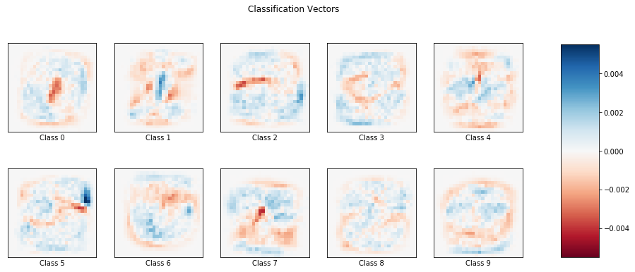
As we have a multi-class problem, the coefficient has shape (number of classes, number of features) = (10, 28 \(\times\) 28). Thus, each coefficient can be demonstrated as an image.

Classification vector \(k\) can be interpreted as follows: if a testing image has a high probability to be classified into class \(k\), comparing to the class \(k\) image below, then we expect to see more pixels at the blue area (high weight) and less pixels at the red area (low weight) in the testing image.

coef = logisticReg.coef_.copy()
scale = np.abs(coef).max()

fig, axes = plt.subplots(nrows=2, ncols=5, figsize=(15,6))
for i, ax in enumerate(axes.flat):
    im = ax.imshow(coef[i].reshape(28, 28), interpolation='nearest',
                   cmap=plt.cm.RdBu, vmin=-scale, vmax=scale)
    ax.set_xticks(())
    ax.set_yticks(())
    ax.set_xlabel('Class %i' % i)

plt.suptitle('Classification Vectors')
fig.subplots_adjust(right=0.8)
cbar_ax = fig.add_axes([0.85, 0.15, 0.05, 0.7])
fig.colorbar(im, cax=cbar_ax)

plt.show()

toggle()

show code

Probit Regression

We have seen that the posterior class probabilities are given by \(f(a)\) where

• \(f\) is a logistic (or softmax) transformation acting on \(a\),

• \(a\) is a linear function of the feature variables.

Is there other way to define \(f(\cdot)\) such that \(f(a) =\) the posterior class probability \(p(t=1|a)\)? To answer the question, we want to model the posterior probability \(p(t=1|a)\) directly instead of using Bayes’ theorem.

Let target value

\begin{align*} t_i = \left\{ \begin{aligned} 1 & \text{ if } a_i=\mathbf{w}^\intercal \mathbf{\phi}_i \ge \theta \\ 0 & \text{ otherwise.} \end{aligned}\right. \end{align*}

If \(\theta\) has a probability density \(p(\theta)\) (assumed to be a standard Gaussian), then

\begin{align*} p(t=1|a) = \int_{-\infty}^{a} p(\theta) d\theta = \int_{-\infty}^{a} \mathcal{N}(\theta|0,1) d\theta = \Phi(a) = \frac{1}{2} \left(1+\frac{1}{\sqrt{2}}\text{erf}(a) \right) \end{align*}

The generalized linear model based on activation function

\begin{align*} f(a) = \frac{1}{2} \left(1+\frac{1}{\sqrt{2}}\text{erf}(a) \right) \end{align*}

is known as probit regression.

• The tails of the logistic sigmoid decay asymptotically like \(\exp(-x)\) for \(x \to \infty\)

• The tails of the probit decay asymptotically like \(\exp(-x^2)\) for \(x \to \infty\)

• The probit model is significantly more sensitive to outliers.

Mislabelling

Both the logistic and the probit models assume the data is correctly labelled. The effect of mislabelling is easily incorporated into a probabilistic model by introducing a probability \(\epsilon\) that the target value \(t\) has been flipped to the wrong value, so

\begin{align*} p(t|\mathbf{x}) = (1-\epsilon) \sigma(\mathbf{x}) + \epsilon (1-\sigma(\mathbf{x})) \end{align*}

where \(\epsilon\) may be set in advance, or it may be treated as a hyperparameter whose value is inferred from the data.

Bayesian Logistic Regression

Exact Bayesian inference for logistic regression is intractable because the posterior distribution comprises a product of logistic sigmoid functions

Posterior Distribution

The posterior distribution over \(\mathbf{w}\) is

\begin{align*} p(\mathbf{w}|\mathbf{t}) \propto p(\mathbf{t}|\mathbf{w})p(\mathbf{w}) \end{align*}

with a Gaussian prior \(p(\mathbf{w}) = \mathcal{N}(\mathbf{w}|\mathbf{m}_0, \mathbf{S}_0)\). From equation (Likelihood),

\begin{align} \ln p(\mathbf{w}|\mathbf{t}) & = -\frac{1}{2} (\mathbf{w}-\mathbf{m}_0)^\intercal \mathbf{S}^{-1}_0 (\mathbf{w}-\mathbf{m}_0) \nonumber \\ & \quad + \sum_{i=1}^{n} \left( t_i \ln y_i + (1-t_i) \ln (1-y_i) \right) + \text{const} \nonumber \end{align}

• The posterior distribution \(p(\mathbf{w}|\mathbf{t})\) is not Gaussian due to the second term.

• We seek a Gaussian representation

\begin{align*} p(\mathbf{w}|\mathbf{t}) = q(\mathbf{w}) \equiv \mathcal{N}(\mathbf{w}_{MAP}, \mathbf{S}_N) \end{align*}

for the posterior distribution by using Laplace approximation.

hide_comment()

show comment

Laplace Approximation is to find a Gaussian approximation to a probability density \(p(z)\)

\begin{align*} p(z) &= \frac{1}{Z} f(z) \text{ where } Z = \int f(z) dz \\ p(z) & \sim \mathcal{N}(z|z_0, A^{-1}) \text{ where $z_0$ is a mode of } p(z) \end{align*}

\(f^\prime (z_0) = 0\) and \(A = - \nabla \nabla \ln f(z_0)\). Laplace framework is based purely on the aspects of the true distribution at mode of the variable, and so can fail to capture important global properties. In Bayesian logistic regression,

\begin{align} \mathbf{S}_N &= -\nabla \nabla \ln p(\mathbf{w}|\mathbf{t}) = \mathbf{S}^{-1}_0 \sum_{i=1}^{n} y_i(1-y_i) \phi_i \phi_{i}^\intercal \nonumber \end{align}

\(\blacksquare\)

Predictive Distribution

The predictive distribution

\begin{align} p(\mathcal{C}_1|\phi,\mathbf{t}) &= \int p(\mathcal{C}_1|\phi,\mathbf{w}) p(\mathbf{w}|\mathbf{t})dw \approxeq \int \sigma(\mathbf{w}^\intercal \phi) q(\mathbf{w}) dw \nonumber \\ &= \int \sigma(a) \left(\int \delta(a-\mathbf{w}^\intercal \phi) q(\mathbf{w})\right) da \equiv \int \sigma(a) p(a) da\nonumber \\ & \approxeq \int \sigma(a) \mathcal{N}(a|\mu_a, \sigma^2_a) da \quad \quad \text{Apply Laplace approximation}\nonumber \end{align}

where \(\delta\) is Dirac function, \(a = \mathbf{w}^\intercal \phi\), and

\begin{align} \mu_a &= E(a) = \int p(a) a da = \int q(\mathbf{w}) \mathbf{w}^\intercal \phi dw = \mathbf{w}^T_{MAP} \phi \nonumber \\ \sigma^2_a &= \text{var}(a) = \int p(a) (a^2 - \mu_a^2) da = \phi^\intercal \mathbf{S}_N \phi \nonumber \end{align}

• The predictive distribution is the convolution of a Gaussian with a logistic sigmoid, and cannot be evaluated analytically,

• We can use probit function \(\Phi\), then the convolution can be expressed analytically.

x1_test, x2_test = np.meshgrid(np.linspace(-5, 12, 100), np.linspace(-5, 12, 100))
x_test = np.array([x1_test, x2_test]).reshape(2, -1).T

funcs = {'Linear Discriminant Analysis':'LinearDiscriminantAnalysis',\
        'Quadratic Discriminant Analysis':'QuadraticDiscriminantAnalysis',\
        'User Logistic':'Logistic', 'Logistic Regression':'LogisticRegression',\
        'Bayesian Ridge':'BayesianRidge'}

from ipywidgets import interact, widgets
widget_layout = widgets.Layout(width='270px', height='30px')
@interact(method = widgets.Dropdown(description='Methods:',\
                                        style = {'description_width': 'initial'},\
                                        options=['User Logistic','Logistic Regression','Linear Discriminant Analysis',\
                                                'Quadratic Discriminant Analysis','Bayesian Ridge'],\
                                        value='User Logistic',\
                                        layout=widget_layout))

def classify(method):
    plt.figure(figsize=(16, 4))
    for i, (key, value) in enumerate(train_data.items()):
        plt.subplot(1, 3, i+1)
        x_train, t_train = value
        t = globals()[funcs[method]]().fit(x_train, t_train).predict(x_test)
        plt.scatter(x_train[:,0], x_train[:,1], c=t_train, cmap=matplotlib.colors.ListedColormap(['red','green','blue']))
        plt.contourf(x1_test, x2_test, t.reshape(100, 100), alpha=0.3, levels=np.array([0., 0.5, 1.5, 2.]),
                    cmap=matplotlib.colors.ListedColormap(['yellow','green','purple']))
        plt.xlim(-5, 12)
        plt.ylim(-5, 12)
        plt.colorbar()
        plt.gca().set_aspect('equal', adjustable='box')
        plt.title("{}".format(key))
    plt.show()

toggle()

show code

Information Criterion

• Akaike information criterion (AIC):

\(\ln p(\mathcal{D}|\mathbf{w}_{\text{ML}}) - M\), where \(p(\mathcal{D}|\mathbf{w}_{\text{ML}})\) is the best-fit log likelihood and \(M\) is number of parameters in \(\theta\).

• Bayesian Information Criterion (BIC):

\(\ln p(\mathcal{D}|\mathbf{w}_{\text{MAP}}) - \frac{1}{2} M \ln n\), where \(n\) is the number of data points.

hide_comment()

show comment

The intuition of Bayesian Information Criterion

Laplace approximate gives

\begin{align} Z &= \int f(\mathbf{z}) d\mathbf{z} \approx f(\mathbf{z}_0) \int \exp \left\{ -\frac{1}{2} (\mathbf{z}-\mathbf{z}_0)^\intercal \mathbf{A} (\mathbf{z} - \mathbf{z}_0)\right\} d\mathbf{z} = f(\mathbf{z}_0) \frac{(2\pi)^{M/2}}{|\mathbf{A}|^{1/2}} \label{eqn_bic} \end{align}

where

\begin{align*} \mathbf{A} = - \nabla \nabla \ln f(\mathbf{z})|_{\mathbf{z} = \mathbf{z}_0} \end{align*}

From Bayes’ theorem, the model evidence is

\begin{align*} p(\mathcal{D}) & = \int p(\mathcal{D}|\theta) p(\theta) d\theta \end{align*}

identifying \(Z = p(\mathcal{D})\) and \(f(\theta) = p(\mathcal{D}|\theta) p(\theta)\)), \eqref{eqn_bic} gives

\begin{align*} \ln p(\mathcal{D}) &\approx \ln p(\mathcal{D}|\mathbf{w}_{\text{MAP}}) + \underbrace{\ln p(\mathbf{w}_{\text{ML}}) + \frac{M}{2} \ln (2\pi) - \frac{1}{2} \ln |A|}_{\text{Occam factor}} \nonumber \\ &\approx \ln p(\mathcal{D}|\mathbf{w}_{\text{MAP}}) - \frac{1}{2} M \ln n \end{align*}

“Occam factor” penalizes model complexity.

\(\blacksquare\)