[1]:
%run initscript.py
%run ./files/loadtsfuncs.py
HTML("""
<div id="popup" style="padding-bottom:5px; display:none;">
    <div>Enter Password:</div>
    <input id="password" type="password"/>
    <button onclick="done()" style="border-radius: 12px;">Submit</button>
</div>
<button onclick="unlock()" style="border-radius: 12px;">Unclock</button>
<a href="#" onclick="code_toggle(this); return false;">show code</a>
""")
[1]:
Times Series Analysis
Forecasting Methods
Forecasting methods can be generally divided into:
Econometric methods
Time series methods
Judgmental Forecasts
Forecasting using judgment is common in practice. In many cases, judgmental forecasting is the only option, such as when there is a complete lack of historical data, or when a new product is being launched, or when a new competitor enters the market, or during completely new and unique market conditions.
Judgmental methods are basically nonquantitative and will not be discussed here. Instead, we will talk about some simple forecasting strategies based on Bayes rule.
Bayes Rule
Bayes Rule can be simply expressed as
\begin{align*} \text{posterior} \propto \text{likelihood} \times \text{prior} \end{align*}
In other words, prediction \(\approx\) observations \(\times\) prior knowledge.
Example: J. Richard Gott III. took a trip to Europe in 1969 and saw the stark symbol of the Cold War — Berlin Wall which had been built eight years earlier in 1961. A question in his mind is “how much longer it would continue to divide the East and West?”.
This may sounds like an absurd prediction. Even setting aside the impossibility of forecasting geopolitics, the question seems mathematically impossible: he needs to make a prediction from a single data point. But as ridiculous as this might seem on its face, we make such predictions all the time by necessity.

John Richard Gott III is a professor of astrophysical sciences at Princeton University.
He is known for developing and advocating two cosmological theories: Time travel and the Doomsday theory.
Gott first thought of his “Copernicus method” of lifetime estimation in 1969 when stopping at the Berlin Wall and wondering how long it would stand.
[2]:
hide_answer()
[2]:
Why it is called the Copernican principle (method)?
In about 1510, the astronomer Nicolaus Copernicus was obsessed by questions: Where are we? Where in the universe is the Earth? Copernicus made a radical imagining at his time that the Earth was not the center of the universe, but, in fact, nowhere special in particular.
When Gott arrived at the Berlin Wall, he asked himself the same question: Where am I? That is to say, where in the total life span of this artifact have I happened to arrive? In a way, he was asking the temporal version of the spatial question that had proposed by Copernicus four hundred years earlier. Gott decided to take the same step with regard to time.
He made the assumption that the moment when he encountered the Berlin Wall was not special. My visit should be located at some random point between the Wall’s beginning and its end. 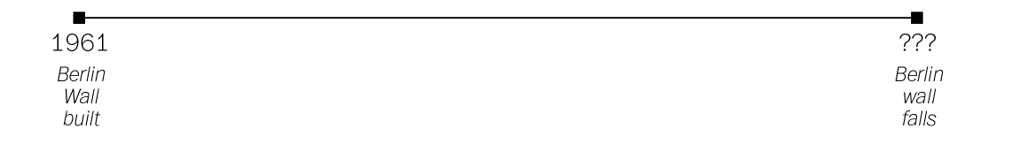
We can divide that timeline up into quarters, like so. 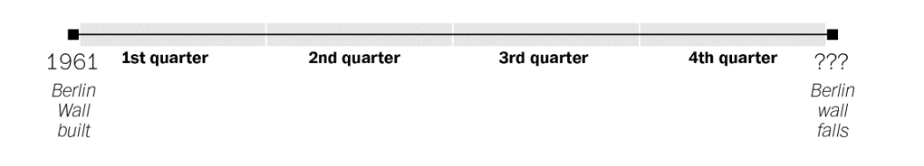
Gott reasoned that his visit, because it was not special in any way, could be located anywhere on that timeline. From the standpoint of probability, that meant there was a 50 percent chance that it was somewhere in the middle portion of the wall’s timeline — the middle two quarters, or 50 percent, of its existence. 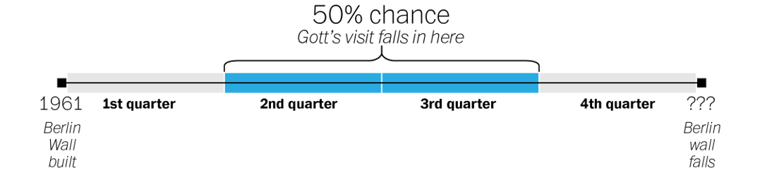
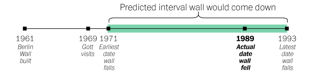
When Gott visited in 1969, the Wall had been standing for eight years. If his visit took place at the very beginning of that middle portion of the Wall’s existence, Gott reasoned, that eight years would represent exactly one quarter of the way into its history. That would mean the Wall would exist for another 24 years, coming down in 1993. 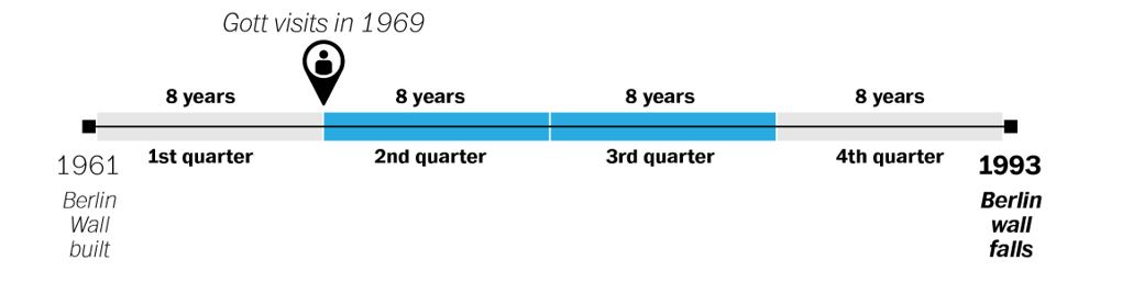
If, on the other hand, his visit happened at the very end of the middle portion, then the eight years would represent exactly three quarters of the way into the Wall’s history. Each quarter would represent just 2.66 years, meaning that the wall could fall as early as 1971. 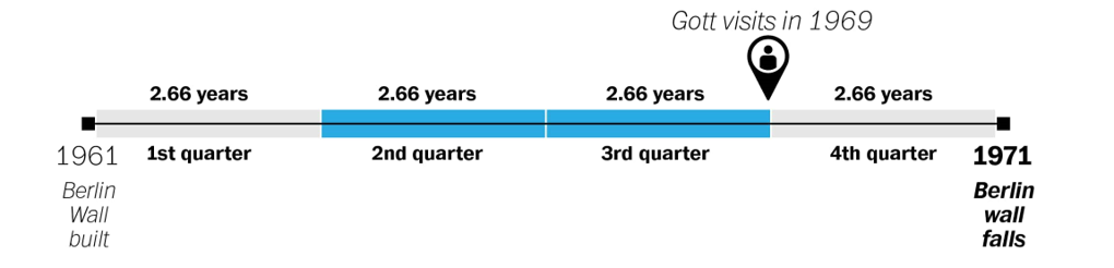
What if we need a single number prediction instead of a range?
Recall that Gott made the assumption that the moment when he encountered the Berlin Wall wasn’t special–that it was equally likely to be any moment in the wall’s total lifetime. And if any moment was equally likely, then on average his arrival should have come precisely at the halfway point (Why? since it was 50% likely to fall before halfway and 50% likely to fall after).
More generally, unless we know better we can expect to have shown up precisely halfway into the duration of any given phenomenon. And if we assume that we’re arriving precisely halfway into the duration, the best guess we can make for how long it will last into the future becomes obvious: exactly as long as it’s lasted already. Since Gott saw Berlin Wall eight years after it was built, so his best guess was that it would stand for eight years more. 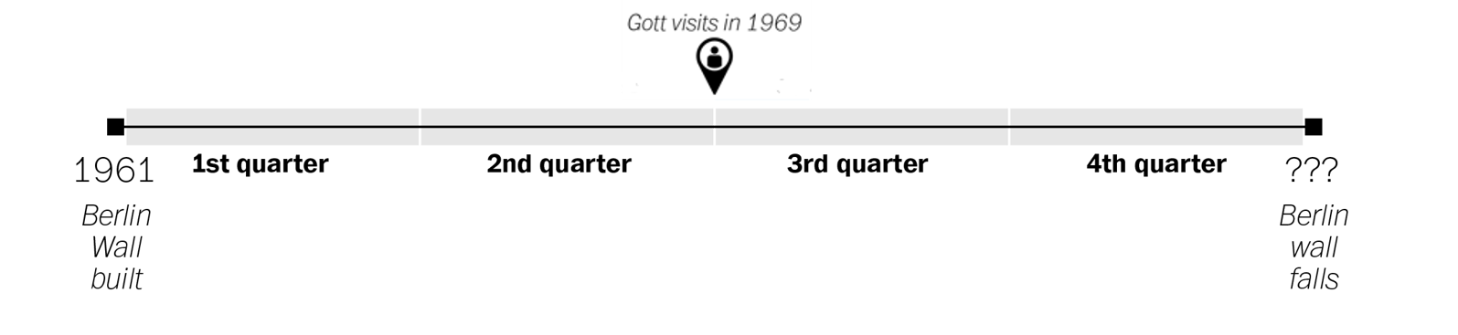
\(\blacksquare\)
Example: You arrive at a bus stop in a foreign city and learn, perhaps, that the other tourist standing there has been waiting 7 minutes. When is the next bus likely to arrive? Is it worthwhile to wait — and if so, how long should you do so before giving up? 
Example: A friend of yours has been dating somebody for ONE Month and wants your advice: is it too soon to invite him/her along to an upcoming family wedding? The relationship is off to a good start, but how far ahead is it safe to make plans? 
One thing in common for all these examples is that we don’t have much information, or even we have some information, how should we incorporate our information into forecasting. Let’s hold those forecasting questions in mind, and start with some simple math.
Example: There are two different coins. One is a fair coin with a 50–50 chance of heads and tails; the other is a two-headed coin. I drop them into a bag and then pull one out at random. Then I flip it once: head. Which coin do you think I flipped? 
[3]:
hide_answer()
[3]:
There is 100% change to get head for two-headed coin, but only 50% for the normal coin. Thus we can assert confidently that it’s exactly twice as probable, that I had pulled out the two headed coin.
\(\blacksquare\)
Now I show you 9 fair coins and 1 two-headed coin, puts all ten into a bag, draws one at random, and flips it: head. Now what do you suppose? Is it a fair coin or the two-headed one? 
[4]:
hide_answer()
[4]:
As before, a fair coin is exactly half as likely to come up heads as a two-headed coin.
But now, a fair coin is also 9 times as likely to have been drawn in the first place.
Its exactly 4.5 times more likely that I am holding a fair coin than the two-headed one.
The number of coins and its probability of showing head are our priors. The outcome of a flip is our observation. We have different predictions when our priors are different.
\(\blacksquare\)
Is the Copernican Principle Right?
After Gott published his conjecture in Nature, the journal received a flurry of critical correspondence. And it’s easy to see why when we try to apply the rule to some more familiar examples. If you meet a 90-year-old man, the Copernican Principle predicts he will live to 180. Every 6-year-old boy, meanwhile, is predicted to face an early death at the age of 12.
The Copernican Principle is exactly the Bayes Rule by using an uninformative prior. The question is what prior we should use.
Some simple prediction rules:
Average Rule: If our prior information follows normal distribution (things that tend toward or cluster around some kind of natural value), we use the distribution’s “natural” average — its single, specific scale — as your guide.
For example, average life span for men in US is 76 years. So, for a 6-year-old boy, the prediction is 77. He gets a tiny edge over the population average of 76 by virtue of having made it through infancy: we know he is not in the distribution’s left tail.
Multiplicative Rule: If our prior information shows that the rare events have tremendous impact (power-law distribution),
then multiply the quantity observed so far by some constant factor.
For example, movie box-office grosses do not cluster to a “natural” center. Instead, most movies don’t make much money at all, but the occasional Titanic makes titanic amounts. Income (or money in general) is also follows the power-laws (the rich get richer).
For the grosses of movies, the multiplier happens to be 1.4. So if you hear a movie has made $6 million so far, you can guess it will make about $8.4 million overall.
This multiplicative rule is a direct consequence of the fact that power-law distributions do not specify (or you are uninformative on) a natural scale for the phenomenon they are describing. It is possible that a movie that is grossed $6 million is actually a blockbuster in its first hour of release, but it is far more likely to be just a single-digit-millions kind of movie.
In summary, something normally distributed that’s gone on seemingly too long is bound to end shortly; but the longer something in a power-law distribution has gone on, the longer you can expect it to keep going.
There’s a third category of things in life: those that are neither more nor less likely to end just because they have gone on for a while.
Additive Rule: If the prior follows Erlang distributions (e.g. exponential or gamma distributions), then we should always predict that things will go on just a constant amount longer. It is a memoryless prediction.
Additive rule is suitable for events that are completely independent from one another and the intervals between them thus fall on Erlang distribution.
If you wait for a win at the roulette wheel, what is your strategy?
[5]:
hide_answer()
[5]:
Suppose a win at the roulette wheel were characterized by a normal distribution, then the Average Rule would apply: after a run of bad luck, it’d tell you that your number should be coming any second, probably followed by more losing spins. The strategy is to quit after winning.
If, instead, the wait for a win obeyed a power-law distribution, then the Multiplicative Rule would tell you that winning spins follow quickly after one another, but the longer a drought had gone on the longer it would probably continue. The strategy is keep playing for a while after any win, but give up after a losing streak.
If it is a memoryless distribution, then you’re stuck. The Additive Rule tells you the chance of a win now is the same as it was an hour ago, and the same as it will be an hour from now. Nothing ever changes. You’re not rewarded for sticking it out and ending on a high note; neither is there a tipping point when you should just cut your losses. For a memoryless distribution, there is no right time to quit. This may in part explain these games’ addictiveness.
In summary, knowing what distribution you’re up against (i.e. having a correct prior knowledge) can make all the difference.
\(\blacksquare\)
Small Data is Big Data in Disguise
Many behavior studies show that the predictions that people had made were extremely close to those produced by Bayes Rule.
The reason we can often make good predictions from a small number of observations — or just a single one — is that our priors are so rich.
Behavior studies show that we actually carry around in our heads surprisingly accurate priors.
However, the challenge has increased with the development of the printing press, the nightly news, and social media. Those innovations allow us to spread information mechanically which may affect our priors.
As sociologist Barry Glassner notes, the murder rate in the United States declined by 20% over the course of the 1990s, yet during that time period the presence of gun violence on American news increased by 600%.
If you want to naturally make good predictions by following your intuitions, without having to think about what kind of prediction rule is appropriate, you need to protect your priors. Counter-intuitively, that might mean turning off the news.
Fitting and Forecasting
We have 12 data points that are generated from \(\sin(2 \pi x)\) with some small perturbations.
[6]:
interact(training_data,
         show=widgets.Checkbox(value=False, description='Original', disabled=False));
Our task is to foresee (forecast) the underlying data pattern, which is \(\sin(2 \pi x)\), based on given 12 observations. Note
The function \(\sin(2 \pi x)\) is the information we are trying to obtain
The perturbations are noises that we do not want to extract
Remember that we only observe training data without knowing anything about underlying generating function \(\sin(2 \pi x)\) and perturbations. Suppose we try to interpret the data by polynomial functions with degree 1 (linear regression), 3 and 9.
[7]:
interact(poly_fit,
         show=widgets.Checkbox(value=True, description='sin$(2\pi x)$', disabled=False));
With knowing the underlying true function \(\sin(2 \pi x)\), it is clear that
the linear regression is under-fitting because it doesn’t explain the up-and-down pattern in the data;
the polynomial function with degree 9 is over-fitting because it focuses too much on noises and does not correctly interpret the pattern in the data;
the polynomial with degree 3 is the best because it balances the information and noises and extracts the valuable information from the data.
However, is it possible to identify that a polynomial with degree 3 is the best without knowing the underlying true function?
Yes. We can use holdout as follows:
choose 3 data points as testing data
fit polynomial functions only on the remaining 9 data points
find the best fitting function based on the testing data
[8]:
interact(poly_fit_holdout,
         show=widgets.Checkbox(value=True, description='sin$(2\pi x)$', disabled=False),
         train=widgets.Checkbox(value=True, description='Training Data', disabled=False),
         test=widgets.Checkbox(value=True, description='Testing Data', disabled=False));
Occam’s razor the law of parsimony: we generally prefer a simpler model because simpler models track only the most basic underlying patterns and can be more flexible and accurate in forecasting the future!
Time Series Data
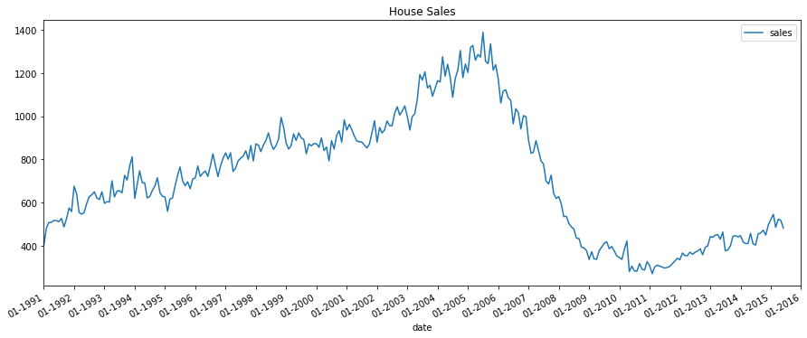
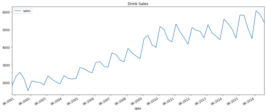
Time series is a sequence of observations recorded at regular time intervals with many applications such as in demand and sales, number of visitors to a website, stock price, etc. In this section, we focus on two time series datasets that one is the US houses sales and the other is the soft drink sales.
The python package pandas is used to read .cvs data file. The first 5 rows are shown as below.
[9]:
df_house.head()
[9]:
| sales | year | month | |
|---|---|---|---|
| date | |||
| 1991-01-01 | 401 | 1991 | Jan |
| 1991-02-01 | 482 | 1991 | Feb |
| 1991-03-01 | 507 | 1991 | Mar |
| 1991-04-01 | 508 | 1991 | Apr |
| 1991-05-01 | 517 | 1991 | May |
[10]:
df_drink.head()
[10]:
| sales | year | quarter | |
|---|---|---|---|
| date | |||
| 2001-03-31 | 1807.37 | 2001 | Q1 |
| 2001-06-30 | 2355.32 | 2001 | Q2 |
| 2001-09-30 | 2591.83 | 2001 | Q3 |
| 2001-12-31 | 2236.39 | 2001 | Q4 |
| 2002-03-31 | 1549.14 | 2002 | Q1 |
There are univariate and multivariate time series where - A univariate time series is a series with a single time-dependent variable, and - A Multivariate time series has more than one time-dependent variable. Each variable depends not only on its past values but also has some dependency on other variables. This dependency is used for forecasting future values.
Our datasets are univariate time series. Time series data can be thought of as special cases of panel data. Panel data (or longitudinal data) also involves measurements over time. The difference is that, in addition to time series, it also contains one or more related variables that are measured for the same time periods.
Now, We plot the time series data
[11]:
plot_time_series(df_house, 'sales', title='House Sales')
[12]:
plot_time_series(df_drink, 'sales', title='Drink Sales')
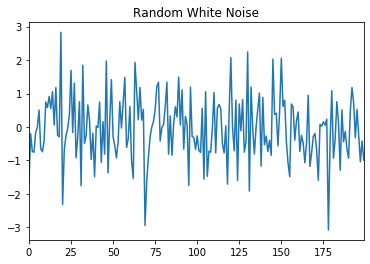
White Noise
A time series is white noise if the observations are independent and identically distributed with a mean of zero. This means that all observations have the same variance and each value has a zero correlation with all other values in the series. White noise is an important concept in time series analysis and forecasting because:
Predictability: if the time series is white noise, then, by definition, it is random. We cannot reasonably model it and make predictions.
Model diagnostics: the series of errors from a time series forecast model should ideally be white noise.
[13]:
pd.Series(np.random.randn(200)).plot(title='Random White Noise')
plt.show()
Random Walk
The series itself is not random. However, its differences - that is, the changes from one period to the next - are random. The random walk model is
and the difference form of random walk model is
where \(\mu\) is the drift. Apparently, the series tends to trend upward if \(\mu > 0\) or downward if \(\mu < 0\).
[14]:
interact(random_walk, drift=widgets.FloatSlider(min=-0.1,max=0.1,step=0.01,value=0,description='Drift:'));
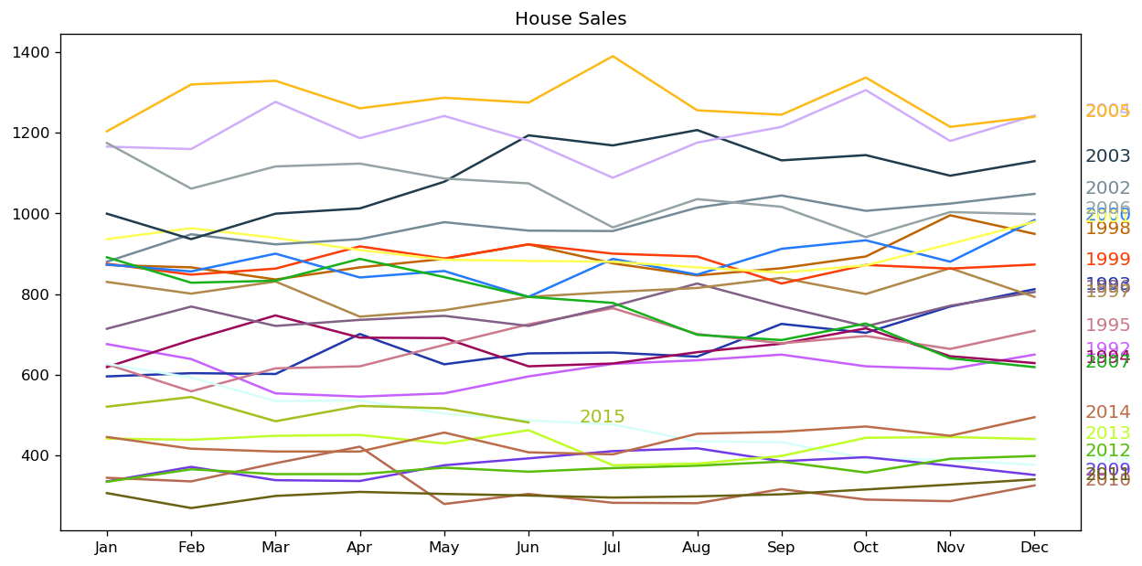
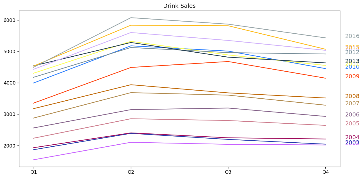
Seasonal Plot
The datasets are either a monthly or quarterly time series. They may follows a certain repetitive pattern every year. So, we can plot each year as a separate line in the same plot. This allows us to compare the year-wise patterns side-by-side.
[15]:
seasonal_plot(df_house, ['month','sales'], title='House Sales')
[16]:
seasonal_plot(df_drink, ['quarter','sales'], title='Drink Sales')
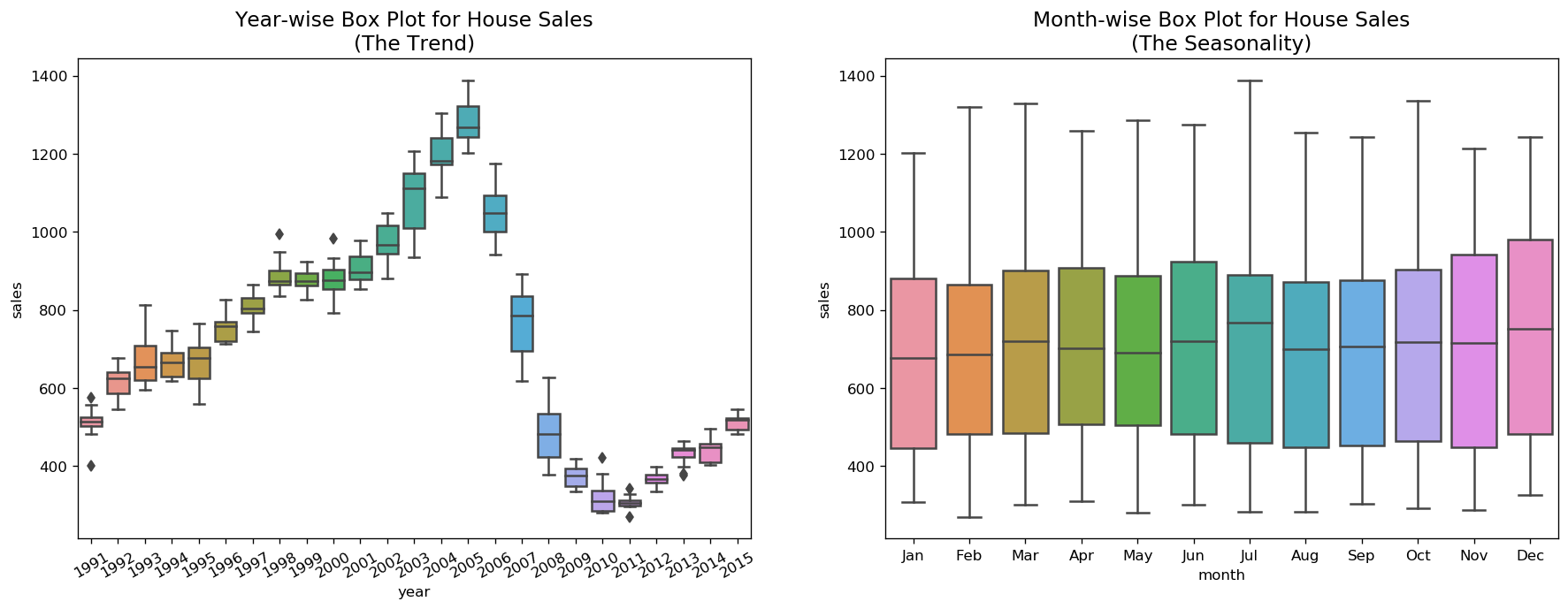
For house sales, we do not see a clear repetitive pattern in each year. It is also difficult to identify a clear trend among years.
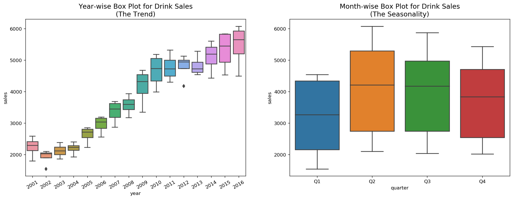
For drink sales, there is a clear pattern repeating every year. It shows a steep increase in drink sales every 2nd quarter. Then, it is falling slightly in the 3rd quarter and so on. As years progress, the drink sales increase overall.
Boxplot of Seasonal and Trend Distribution
We can visualize the trend and how it varies each year in a year-wise or month-wise boxplot for house sales, as well as quarter-wise boxplot for drink sales.
[17]:
boxplot(df_house, ['month','sales'], title='House Sales')
[18]:
boxplot(df_drink, ['quarter','sales'], title='Drink Sales')
Smoothen a Time Series
Smoothening of a time series may be useful in: - Reducing the effect of noise in a signal get a fair approximation of the noise-filtered series. - The smoothed version of series can be used as a feature to explain the original series itself. - Visualize the underlying trend better
Moving average smoothing is certainly the most common smoothening method.
[19]:
interact(moving_average, span=widgets.IntSlider(min=3,max=30,step=3,value=6,description='Span:'));
There are other methods such as LOESS smoothing (LOcalized regrESSion) and LOWESS smoothing (LOcally Weighted regrESSion).
LOESS fits multiple regressions in the local neighborhood of each point. It is implemented in the statsmodels package, where we can control the degree of smoothing using frac argument which specifies the percentage of data points nearby that should be considered to fit a regression model.
[20]:
interact(lowess_smooth, frac=widgets.FloatSlider(min=0.05,max=0.3,step=0.05,value=0.05,description='Frac:'));
Forecasting with Regression
Many time series follow a long-term trend except for random variation which can be modeled by regression:
\begin{equation*} Y_t = a + b t + e_t \end{equation*}
Example: Monthly US population.
[21]:
df = pd.read_csv(dataurl+'Regression1.csv', parse_dates=['Month'], header=0, index_col='Month')
plot_time_series(df, 'Population', freq='', title='')
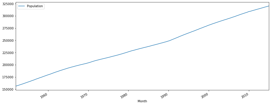
The plot indicates a clear upward trend with little or no curvature. Therefore, a linear trend is plausible.
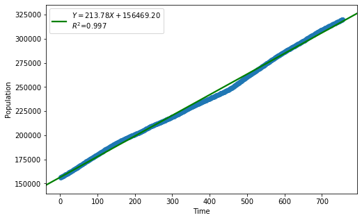
[22]:
df = pd.read_csv(dataurl+'Regression1.csv', parse_dates=['Month'], header=0, index_col='Month')
_ = analysis(df, 'Population', ['Time'], printlvl=4)
| Dep. Variable: | Population | R-squared: | 0.997 |
|---|---|---|---|
| Model: | OLS | Adj. R-squared: | 0.997 |
| Method: | Least Squares | F-statistic: | 2.467e+05 |
| Date: | Thu, 22 Aug 2019 | Prob (F-statistic): | 0.00 |
| Time: | 10:02:36 | Log-Likelihood: | -7011.3 |
| No. Observations: | 756 | AIC: | 1.403e+04 |
| Df Residuals: | 754 | BIC: | 1.404e+04 |
| Df Model: | 1 | ||
| Covariance Type: | nonrobust |
| coef | std err | t | P>|t| | [0.025 | 0.975] | |
|---|---|---|---|---|---|---|
| Intercept | 1.565e+05 | 188.045 | 832.084 | 0.000 | 1.56e+05 | 1.57e+05 |
| Time | 213.7755 | 0.430 | 496.693 | 0.000 | 212.931 | 214.620 |
| Omnibus: | 112.704 | Durbin-Watson: | 0.000 |
|---|---|---|---|
| Prob(Omnibus): | 0.000 | Jarque-Bera (JB): | 67.588 |
| Skew: | -0.600 | Prob(JB): | 2.11e-15 |
| Kurtosis: | 2.160 | Cond. No. | 875. |
Warnings:
[1] Standard Errors assume that the covariance matrix of the errors is correctly specified.
standard error of estimate:2582.62518
KstestResult(statistic=0.5674603174603174, pvalue=1.6534900647623363e-230)
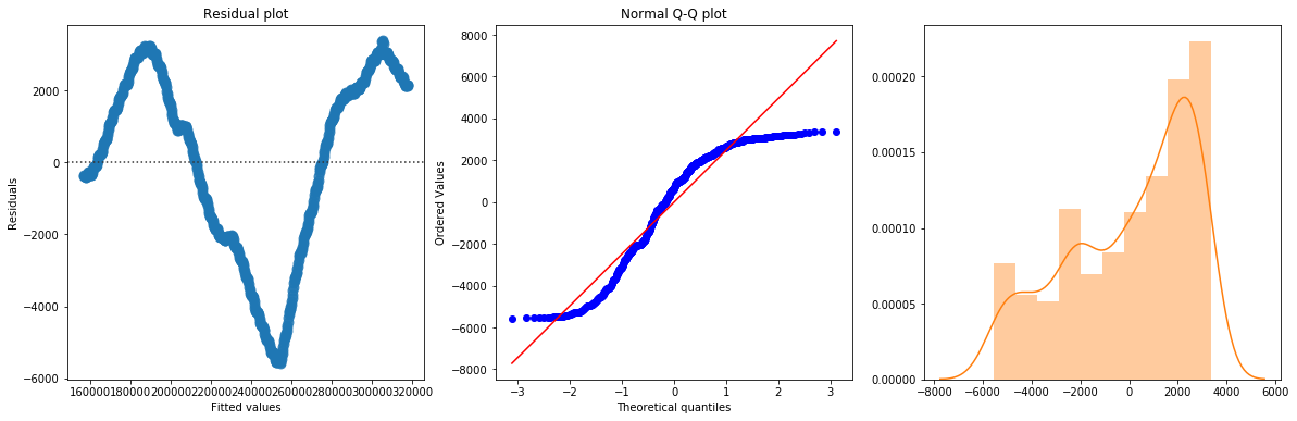
The linear fit has a very high R-squared, but is not perfect, as the residual plot indicates.
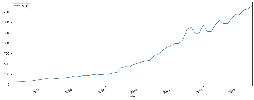
Example: Quarterly PC device sales.
[23]:
df_reg = pd.read_csv(dataurl+'Regression2.csv', parse_dates=['Quarter'], header=0)
df_reg['date'] = [pd.to_datetime(''.join(df_reg.Quarter.str.split('-')[i][-1::-1]))
                       + pd.offsets.QuarterEnd(0) for i in df_reg.index]
df_reg = df_reg.set_index('date')

plot_time_series(df_reg, 'Sales', freq='', title='')
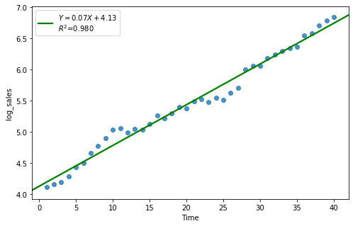
[24]:
df_reg['log_sales'] = np.log(df_reg['Sales'])
df_reg[:40].tail()
[24]:
| Quarter | Sales | Time | log_sales | |
|---|---|---|---|---|
| date | ||||
| 2010-12-31 | Q4-2010 | 700.19 | 36 | 6.551352 |
| 2011-03-31 | Q1-2011 | 723.98 | 37 | 6.584764 |
| 2011-06-30 | Q2-2011 | 821.90 | 38 | 6.711619 |
| 2011-09-30 | Q3-2011 | 889.26 | 39 | 6.790390 |
| 2011-12-31 | Q4-2011 | 935.33 | 40 | 6.840899 |
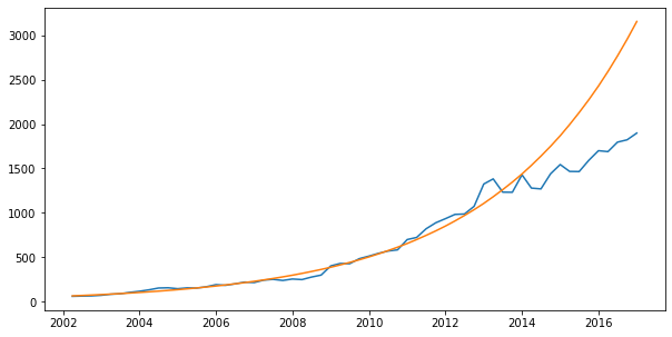
[25]:
result = analysis(df_reg[:40], 'log_sales', ['Time'], printlvl=4)
df_reg['forecast'] = np.exp(df_reg['Time']*result.params[1] + result.params[0])
| Dep. Variable: | log_sales | R-squared: | 0.980 |
|---|---|---|---|
| Model: | OLS | Adj. R-squared: | 0.980 |
| Method: | Least Squares | F-statistic: | 1871. |
| Date: | Thu, 22 Aug 2019 | Prob (F-statistic): | 6.24e-34 |
| Time: | 10:02:37 | Log-Likelihood: | 32.394 |
| No. Observations: | 40 | AIC: | -60.79 |
| Df Residuals: | 38 | BIC: | -57.41 |
| Df Model: | 1 | ||
| Covariance Type: | nonrobust |
| coef | std err | t | P>|t| | [0.025 | 0.975] | |
|---|---|---|---|---|---|---|
| Intercept | 4.1302 | 0.036 | 116.035 | 0.000 | 4.058 | 4.202 |
| Time | 0.0654 | 0.002 | 43.252 | 0.000 | 0.062 | 0.069 |
| Omnibus: | 0.388 | Durbin-Watson: | 0.415 |
|---|---|---|---|
| Prob(Omnibus): | 0.824 | Jarque-Bera (JB): | 0.062 |
| Skew: | -0.090 | Prob(JB): | 0.969 |
| Kurtosis: | 3.071 | Cond. No. | 48.0 |
Warnings:
[1] Standard Errors assume that the covariance matrix of the errors is correctly specified.
standard error of estimate:0.11045
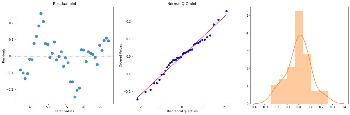
KstestResult(statistic=0.40296611566774143, pvalue=2.228416605814664e-06)
[26]:
plt.subplots(1, 1, figsize=(10,5))
plt.plot(df_reg.index, df_reg.Sales, df_reg.forecast)
plt.show()
Exponential Smoothing Forecasts
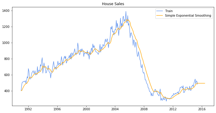
Simple Exponential Smoothing
The simple exponential smoothing method is defined by the following two equations, where
\(L_t\), called the level of the series at time \(t\), is not observable but can only be estimated. Essentially, it is an estimate of where the series would be at time \(t\) if there were no random noise.
\(F_{t+k}\) is the forecast of \(Y_{t+k}\) made at time \(t\).
\begin{align} L_t &= \alpha Y_t + (1-\alpha) L_{t-1} \tag{1}\\ F_{t+k} &= L_t \nonumber \end{align}
The level \(\alpha \in [0,1]\). If you want the method to react quickly to movements in the series, you should choose a large \(\alpha\); otherwise a small \(\alpha\).
If \(\alpha\) is close to 0, observations from the distant past continue to have a large influence on the next forecast. This means that the graph of the forecasts will be relatively smooth.
If \(\alpha\) is close to 1, only very recent observations have much influence on the next forecast. In this case, forecasts react quickly to sudden changes in the series.
Simple exponential smoothing offers “flat” forecasts. That is, all forecasts take the same value, equal to the last level component. Remember that these forecasts will only be suitable if the time series has no trend or seasonal component.
Why exponential smoothing?
Note that
\begin{align} L_{t-1} &= \alpha Y_{t-1} + (1-\alpha) L_{t-2} \tag{2} \\ \end{align}
By substituting equation (2) into equation (1), we get
\begin{align*} L_{t} &= \alpha Y_{t-1} + (1-\alpha) \big( \alpha Y_{t-1} + (1-\alpha) L_{t-2} \big) \\ &= \alpha Y_{t-1} + \alpha(1-\alpha) Y_{t-1} + (1-\alpha)^2 L_{t-2} \end{align*}
If we substitute recursively into the equation (1), we obtain
\begin{align*} L_{t} &= \alpha Y_{t-1} + \alpha(1-\alpha) Y_{t-1} + \alpha(1-\alpha)^2 Y_{t-2} + \alpha(1-\alpha)^3 Y_{t-3} + \cdots \end{align*}
where exponentially decaying weights are assigned to historical data.
[27]:
widgets.interact_manual.opts['manual_name'] = 'Run Forecast'
interact_manual(ses_forecast,
         forecasts=widgets.BoundedIntText(value=12, min=1, description='Forecasts:', disabled=False),
         holdouts=widgets.BoundedIntText(value=0, min=0, description='Holdouts:', disabled=False),
         level=widgets.BoundedFloatText(value=0.2, min=0, max=1, step=0.05, description='Level:', disabled=False),
         optimized=widgets.Checkbox(value=False, description='Optimize Parameters', disabled=False));

ses_forecast(12,0,0.2,False)
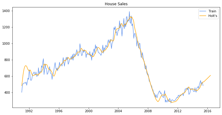
Holt’s Model for Trend
Holt extended simple exponential smoothing to allow the forecasting of data with a trend. This method involves a forecast equation and two smoothing equations where one for the level and one for the trend.
Besides the smoothing constant \(\alpha\) for the level, Holt’s requires a new smoothing constant \(\beta\) for the trend to control how quickly the method reacts to observed changes in the trend.
If \(\beta\) is small, the method reacts slowly,
If \(\beta\) is large, the method reacts more quickly.
Some practitioners suggest using a small value of \(\alpha\) (such as 0.1 to 0.2) and setting \(\beta = \alpha\). Others suggest using an optimization option to select the optimal smoothing constant.
[28]:
from statsmodels.tsa.holtwinters import Holt

# df_house.index.freq = 'MS'
plt.figure(figsize=(12, 6))
train = df_house.iloc[:, 0]
train.index = pd.DatetimeIndex(train.index.values, freq=train.index.inferred_freq)
model = Holt(train).fit(smoothing_level=0.2, smoothing_slope=0.2, optimized=False)
pred = model.predict(start=train.index[0], end=train.index[-1] + 12*train.index.freq)

plt.plot(train.index, train, label='Train', c='cornflowerblue')
plt.plot(pred.index, pred, label='Holt\'s', c='orange')
plt.legend(loc='best')
plt.title('House Sales')
plt.show()

toggle()
[28]:
Damped Trend Methods
The forecasts generated by Holt’s linear method display a constant trend (increasing or decreasing) indefinitely into the future. Empirical evidence indicates that these methods tend to over-forecast, especially for longer forecast horizons. Motivated by this observation, Gardner & McKenzie introduced a parameter that “dampens” the trend to a flat line some time in the future. Methods that include a damped trend have proven to be very successful, and are arguably the most popular individual methods when forecasts are required automatically for many series.
Holt(train, exponential=False, damped=True).fit(...,damping_slope=)
In practice, the damping factor is rarely less than 0.8 as the damping has a very strong effect for smaller values. The damping factor close to 1 will mean that a damped model is not able to be distinguished from a non-damped model. For these reasons, we usually restrict the damping factor to a minimum of 0.8 and a maximum of 0.98.
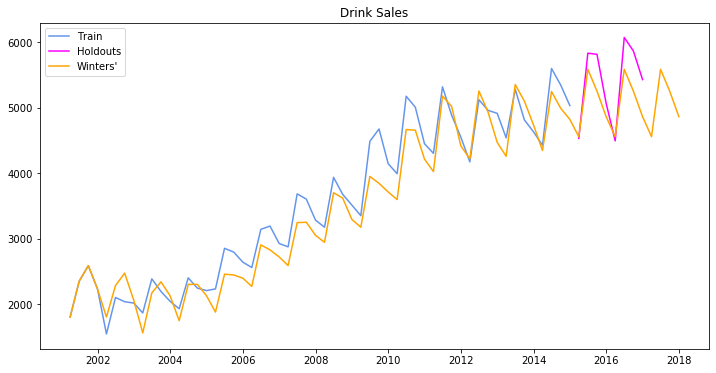
Winters’ Exponential Smoothing Model
The Holt-Winters seasonal method comprises the forecast equation and three smoothing equations: one for the level, one for the trend, and one for the seasonal component.
We use \(m\) to denote the frequency of the seasonality, i.e., the number of seasons in a year. For example, for quarterly data \(m = 4\), and for monthly data \(m=12\). There are two variations to this method that differ in the nature of the seasonal component.
The additive method is preferred when the seasonal variations are roughly constant through the series. With the additive method, the seasonal component is expressed in absolute terms in the scale of the observed series, and in the level equation the series is seasonally adjusted by subtracting the seasonal component. Within each year, the seasonal component will add up to approximately zero.
The multiplicative method is preferred when the seasonal variations are changing proportional to the level of the series. With the multiplicative method, the seasonal component is expressed in relative terms (percentages), and the series is seasonally adjusted by dividing through by the seasonal component. Within each year, the seasonal component will sum up to approximately \(m\) (average to 1).
[29]:
from statsmodels.tsa.holtwinters import ExponentialSmoothing

plt.figure(figsize=(12, 6))
train, test = df_drink.iloc[:-8, 0], df_drink.iloc[-8:,0]
train.index = pd.DatetimeIndex(train.index.values, freq=train.index.inferred_freq)

model = ExponentialSmoothing(train, seasonal='mul', seasonal_periods=4).fit(smoothing_level=0.2,
                                        smoothing_slope=0.2,
                                        smoothing_seasonal=0.4,
                                        optimized=False)
pred = model.predict(start=train.index[0], end=test.index[-1] + 4*train.index.freq)

plt.plot(train.index, train, label='Train', c='cornflowerblue')
plt.plot(test.index, test, label='Holdouts', c='fuchsia')
plt.plot(pred.index, pred, label='Winters\'', c='orange')
plt.legend(loc='best')
plt.title('Drink Sales')
plt.show()

toggle()
[29]:
Holt-Winters’ damped method
Damping is possible with both additive and multiplicative Holt-Winters’ methods. A method that often provides accurate and robust forecasts for seasonal data is the Holt-Winters method with a damped trend and multiplicative seasonality
Stationarity
A time series is stationary if the values of the series is not a function of time. Therefore, A stationary time series has constant mean and variance. More importantly, the correlation of the series with its previous values (lags) is also constant. The correlation is called Autocorrelation.
The mean of the series should not be a function of time. The red graph below is not stationary because the mean increases over time.
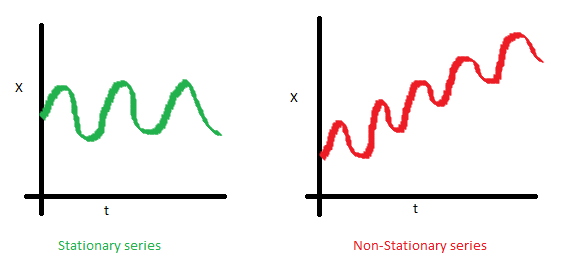
The variance of the series should not be a function of time. This property is known as homoscedasticity. Notice in the red graph the varying spread of data over time.
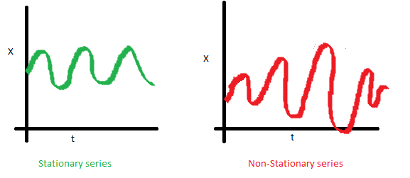
Finally, the covariance of the \(i\)th time and the \((i + m)\)th time should not be a function of time. In the following graph, we notice the spread becomes closer as the time increases. Hence, the covariance is not constant with time for the ‘red series’. 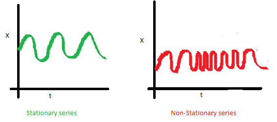
For example, white noise is a stationary series. However, random walk is always non-stationary because of its variance depends on time.
How to Make a Time Series Stationary?
It is possible to make nearly any time series stationary by applying a suitable transformation. The first step in the forecasting process is typically to do some transformation to convert a non-stationary series to stationary. The transformation includes 1. Differencing the Series (once or more) 2. Take the log of the series 3. Take the nth root of the series 4. Combination of the above
The most common and convenient method to stationarize a series is by differencing. Let \(Y_t\) be the value at time \(t\), the fist difference of \(Y\) is \(Y_t - Y_{t-1}\), i.e., subtracting the next value by the current value. If the first difference does not make a series stationary, we can apply the second differencing, and so on.
[30]:
Y = [1, 5, 8, 3, 15, 20]
print('Y = {}\nFirst differencing is {}, Second differencing is {}'.format(Y, np.diff(Y,1), np.diff(Y,2)))
toggle()
Y = [1, 5, 8, 3, 15, 20]
First differencing is [ 4  3 -5 12  5], Second differencing is [-1 -8 17 -7]
[30]:
Why does a Stationary Series Matter?
Most statistical forecasting methods are designed to work on a stationary time series.
Forecasting a stationary series is relatively easy and the forecasts are more reliable.
An important reason is, autoregressive forecasting models are essentially linear regression models that utilize the lag(s) of the series itself as predictors.
We know that linear regression works best if the predictors (\(X\) variables) are not correlated against each other. So, stationarizing the series solves this problem since it removes any persistent autocorrelation, thereby making the predictors(lags of the series) in the forecasting models nearly independent.
Test for Stationarity
The most commonly used is the Augmented Dickey Fuller (ADF) test, where the null hypothesis is the time series possesses a unit root and is non-stationary. So, if the P-Value in ADH test is less than the significance level (for example 5%), we reject the null hypothesis.
The KPSS test, on the other hand, is used to test for trend stationarity. If \(Y_t\) is a trend-stationary process, then
where: - \(\mu_t\) is a deterministic mean trend, - \(e_t\) is a stationary stochastic process with mean zero.
For the KPSS test, the null hypothesis and the P-Value interpretation is just the opposite of ADH test. The below code implements these two tests using statsmodels package in python.
[31]:
stationarity_test(df_house.sales, title='House Sales')
Test on House Sales:

ADF Statistic   : -1.72092
p-value         : 0.42037
Critial Values  :
        1.0%    : -3.45375
        5.0%    : -2.87184
        10.0%   : -2.57226

H0: The time series is non-stationary
We do not reject the null hypothesis.

KPSS Statistic  : 0.50769
p-value         : 0.03993
Critial Values  :
        10.0%   : 0.34700
        5.0%    : 0.46300
        2.5%    : 0.57400
        1.0%    : 0.73900

H0: The time series is stationary
We reject the null hypothesis at 5% level.
[32]:
stationarity_test(df_drink.sales, title='Drink Sales')
Test on Drink Sales:

ADF Statistic   : -0.83875
p-value         : 0.80747
Critial Values  :
        1.0%    : -3.55527
        5.0%    : -2.91573
        10.0%   : -2.59567

H0: The time series is non-stationary
We do not reject the null hypothesis.

KPSS Statistic  : 0.62519
p-value         : 0.02035
Critial Values  :
        10.0%   : 0.34700
        5.0%    : 0.46300
        2.5%    : 0.57400
        1.0%    : 0.73900

H0: The time series is stationary
We reject the null hypothesis at 5% level.
Forecastability
Estimate the Forecastability
The more regular and repeatable patterns a time series has, the easier it is to forecast.
The Approximate Entropy can be used to quantify the regularity and unpredictability of fluctuations in a time series. The higher the approximate entropy, the more difficult it is to forecast it.
A better alternate is the Sample Entropy. Sample Entropy is similar to approximate entropy but is more consistent in estimating the complexity even for smaller time series. For example, a random time series with fewer data points can have a lower approximate entropy than a more regular time series, whereas, a longer random time series will have a higher approximate entropy.
[33]:
# https://en.wikipedia.org/wiki/Approximate_entropy
rand_small = np.random.randint(0, 100, size=50)
rand_big = np.random.randint(0, 100, size=150)

def ApproxEntropy(U, m, r):
    """Compute Aproximate entropy"""
    def _maxdist(x_i, x_j):
        return max([abs(ua - va) for ua, va in zip(x_i, x_j)])

    def _phi(m):
        x = [[U[j] for j in range(i, i + m - 1 + 1)] for i in range(N - m + 1)]
        C = [len([1 for x_j in x if _maxdist(x_i, x_j) <= r]) / (N - m + 1.0) for x_i in x]
        return (N - m + 1.0)**(-1) * sum(np.log(C))

    N = len(U)
    return abs(_phi(m+1) - _phi(m))

print("House data\t: {:.2f}".format(ApproxEntropy(df_house.sales, m=2, r=0.2*np.std(df_house.sales))))
print("Drink data\t: {:.2f}".format(ApproxEntropy(df_drink.sales, m=2, r=0.2*np.std(df_drink.sales))))
print("small size random integer\t: {:.2f}".format(ApproxEntropy(rand_small, m=2, r=0.2*np.std(rand_small))))
print("large size random integer\t: {:.2f}".format(ApproxEntropy(rand_big, m=2, r=0.2*np.std(rand_big))))

toggle()
House data      : 0.53
Drink data      : 0.55
small size random integer       : 0.21
large size random integer       : 0.70
[33]:
The random data should be more difficult to forecast. However, small size data can have small approximate entropy.
[34]:
# https://en.wikipedia.org/wiki/Sample_entropy
def SampleEntropy(U, m, r):
    """Compute Sample entropy"""
    def _maxdist(x_i, x_j):
        return max([abs(ua - va) for ua, va in zip(x_i, x_j)])

    def _phi(m):
        x = [[U[j] for j in range(i, i + m - 1 + 1)] for i in range(N - m + 1)]
        C = [len([1 for j in range(len(x)) if i != j and _maxdist(x[i], x[j]) <= r]) for i in range(len(x))]
        return sum(C)

    N = len(U)
    return -np.log(_phi(m+1) / _phi(m))

print("House sales data\t: {:.2f}".format(SampleEntropy(df_house.sales, m=2, r=0.2*np.std(df_house.sales))))
print("Drink sales data\t: {:.2f}".format(SampleEntropy(df_drink.sales, m=2, r=0.2*np.std(df_drink.sales))))
print("small size random integer\t: {:.2f}".format(SampleEntropy(rand_small, m=2, r=0.2*np.std(rand_small))))
print("large size random integer\t: {:.2f}".format(SampleEntropy(rand_big, m=2, r=0.2*np.std(rand_big))))

toggle()
House sales data        : 0.44
Drink sales data        : 1.03
small size random integer       : 2.30
large size random integer       : 2.41
[34]:
Sample Entropy handles the problem nicely and shows that random data is difficult to forecast.
Granger Causality Test
Granger causality test is used to determine if one time series will be useful to forecast another. The idea is that if \(X\) causes \(Y\), then the forecast of \(Y\) based on previous values of \(Y\) AND the previous values of \(X\) should outperform the forecast of \(Y\) based on previous values of \(Y\) alone.
Therefore, Granger causality should not be used to test if a lag of \(Y\) causes \(Y\). Instead, it is generally used on exogenous (not \(Y\) lag) variables only.
The null hypothesis is: the series in the second column does not Granger cause the series in the first. If the P-Values are less than a significance level (for example 5%) then you reject the null hypothesis and conclude that the said lag of \(X\) is indeed useful. The second argument maxlag says till how many lags of \(Y\) should be included in the test.
[35]:
# https://en.wikipedia.org/wiki/Granger_causality
from statsmodels.tsa.stattools import grangercausalitytests

df_house['m'] = df_house.index.month
# The values are in the first column and the predictor (X) is in the second column.
_ = grangercausalitytests(df_house[['sales', 'm']], maxlag=2)
toggle()
Granger Causality
number of lags (no zero) 1
ssr based F test:         F=0.1690  , p=0.6813  , df_denom=290, df_num=1
ssr based chi2 test:   chi2=0.1708  , p=0.6794  , df=1
likelihood ratio test: chi2=0.1707  , p=0.6795  , df=1
parameter F test:         F=0.1690  , p=0.6813  , df_denom=290, df_num=1

Granger Causality
number of lags (no zero) 2
ssr based F test:         F=0.6936  , p=0.5006  , df_denom=287, df_num=2
ssr based chi2 test:   chi2=1.4115  , p=0.4938  , df=2
likelihood ratio test: chi2=1.4081  , p=0.4946  , df=2
parameter F test:         F=0.6936  , p=0.5006  , df_denom=287, df_num=2
[35]:
[36]:
df_drink['q'] = df_drink.index.quarter
_ = grangercausalitytests(df_drink[['sales', 'q']], maxlag=2)
toggle()
Granger Causality
number of lags (no zero) 1
ssr based F test:         F=74.3208 , p=0.0000  , df_denom=60, df_num=1
ssr based chi2 test:   chi2=78.0368 , p=0.0000  , df=1
likelihood ratio test: chi2=50.7708 , p=0.0000  , df=1
parameter F test:         F=74.3208 , p=0.0000  , df_denom=60, df_num=1

Granger Causality
number of lags (no zero) 2
ssr based F test:         F=108.5323, p=0.0000  , df_denom=57, df_num=2
ssr based chi2 test:   chi2=236.1053, p=0.0000  , df=2
likelihood ratio test: chi2=97.3594 , p=0.0000  , df=2
parameter F test:         F=108.5323, p=0.0000  , df_denom=57, df_num=2
[36]:
For the drink sales data, the P-Values are 0 for all tests. So the quarter indeed can be used to forecast drink sales.
Components of Time Series
Depending on the nature of the trend and seasonality, we have
Additive Model:
\[\text{Data = Seasonal effect + Trend-Cyclical + Residual}\]Multiplicative Model:
\[\text{Data = Seasonal effect $\times$ Trend-Cyclical $\times$ Residual}\]
Note a multiplicative model is additive after a logrithmic transform because
Besides trend, seasonality and error, another aspect to consider is the cyclic behaviour. It happens when the rise and fall pattern in the series does not happen in fixed calendar-based intervals. Care should be taken to not confuse ‘cyclic’ effect with ‘seasonal’ effect.
Cyclic vs Seasonal Pattern
A seasonal pattern exists when a series is influenced by seasonal factors (e.g., the quarter of the year, the month, or day of the week). Seasonality is always of a fixed and known period.
A seasonal behavior is very strictly regular, meaning there is a precise amount of time between the peaks and troughs of the data. For instance temperature would have a seasonal behavior. The coldest day of the year and the warmest day of the year may move (because of factors other than time than influence the data) but you will never see drift over time where eventually winter comes in June in the northern hemisphere.
A cyclic pattern exists when data exhibit rises and falls that are not of fixed period.
Cyclical behavior on the other hand can drift over time because the time between periods isn’t precise. For example, the stock market tends to cycle between periods of high and low values, but there is no set amount of time between those fluctuations.
Some examples about cyclic vs seasonal pattern:
[37]:
hide_answer()
[37]:
Series can show both cyclical and seasonal behavior.
Considering the home prices, there is a cyclical effect due to the market, but there is also a seasonal effect because most people would rather move in the summer when their kids are between grades of school.
You can also have multiple seasonal (or cyclical) effects.
For example, people tend to try and make positive behavioral changes on the “1st” of something, so you see spikes in gym attendance of course on the 1st of the year, but also the first of each month and each week, so gym attendance has yearly, monthly, and weekly seasonality.
When you are looking for a second seasonal pattern or a cyclical pattern in seasonal data, it can help to take a moving average at the higher seasonal frequency to remove those seasonal effects. For instance, if you take a moving average of the housing data with a window size of 12 you will see the cyclical pattern more clearly. This only works though to remove a higher frequency pattern from a lower frequency one.
Seasonal behavior does not have to happen only on sub-year time units.
For example, the sun goes through what are called “solar cycles” which are periods of time where it puts out more or less heat. This behavior shows a seasonality of almost exactly 11 years, so a yearly time series of the heat put out by the sun would have a seasonality of 11.
In many cases the difference in seasonal vs cyclical behavior can be known or measured with reasonable accuracy by looking at the regularity of the peaks in your data and looking for a drift the timing peaks from the mean distance between them.
A series with strong seasonality will show clear peaks in the partial auto-correlation function as well as the auto-correlation function, whereas a cyclical series will only have the strong peaks in the auto-correlation function.
However if you don’t have enough data to determine this or if the data is very noisy making the measurements difficult, the best way to determine if a behavior is cyclical or seasonal can be thinking about the cause of the fluctuation in the data.
If the cause is dependent directly on time then the data are likely seasonal (ex. it takes ~365.25 days for the earth to travel around the sun, the position of the earth around the sun effects temperature, therefore temperature shows a yearly seasonal pattern).
If on the other hand, the cause is based on previous values of the series rather than directly on time, the series is likely cyclical (ex. when the value of stocks go up, it gives confidence in the market, so more people invest making prices go up, and vice versa, therefore stocks show a cyclical pattern).
The class of exponential smoothing allows for seasonality but not cyclicity. The class of ARMA models can handle both seasonality and cyclic behavior, but long-period cyclicity is not handled very well in the ARMA framework.
\(\blacksquare\)
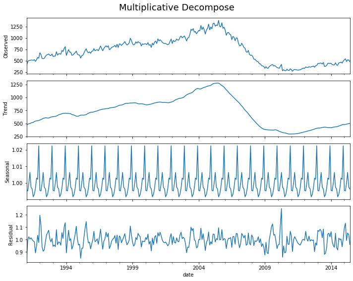
Decompose a Time Series
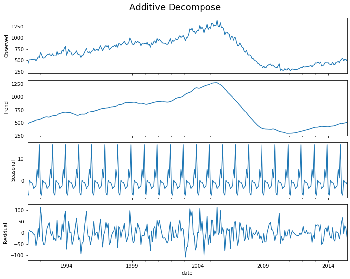
[38]:
decomp(df_house.sales)
Multiplicative Model    : Observed 401.000 = (Seasonal 479.897 * Trend 0.996 * Resid 0.839)
Additive Model          : Observed 401.000 = (Seasonal 479.897 + Trend -5.321 + Resid -73.576)
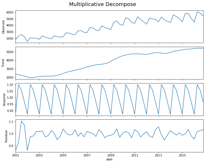
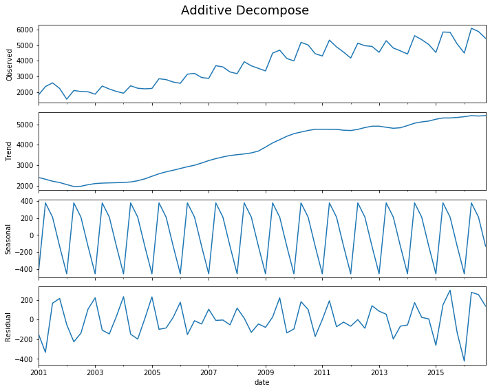
[39]:
decomp(df_drink.sales)
Multiplicative Model    : Observed 1807.370 = (Seasonal 2401.083 * Trend 0.875 * Resid 0.861)
Additive Model          : Observed 1807.370 = (Seasonal 2401.083 + Trend -452.058 + Resid -141.655)
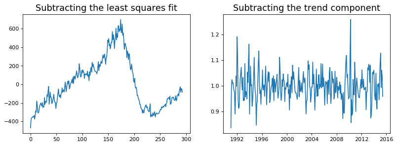
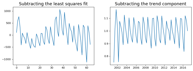
Detrend a Time Series
There are multiple approaches to remove the trend component from a time series:
Subtract the line of best fit from the time series. The line of best fit may be obtained from a linear regression model with the time steps as the predictor. For more complex trends, we can also add quadratic terms \(x^2\) in the model.
Subtract the trend component obtained from time series decomposition we saw earlier.
Subtract the mean
We implement the first two methods. It is clear that the line of best fit is not enough to detrend the data.
[40]:
detrend(df_house['sales'])
[41]:
detrend(df_drink['sales'])
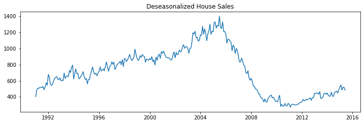
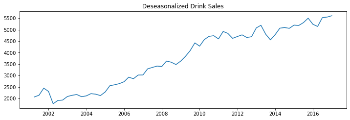
Deseasonalize a Time Series
There are multiple approaches to deseasonalize a time series: 1. Take a moving average with length as the seasonal window. This will smoothen in series in the process. 2. Seasonal difference the series (subtract the value of previous season from the current value) 3. Divide the series by the seasonal index obtained from STL decomposition
If dividing by the seasonal index does not work well, try taking a log of the series and then do the deseasonalizing. You can later restore to the original scale by taking an exponential.
[42]:
deseasonalize(df_house.sales, model='multiplicative', title='House Sales')
[43]:
deseasonalize(df_drink.sales, model='multiplicative', title='Drink Sales')
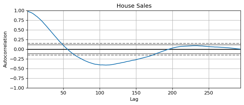
Test for Seasonality
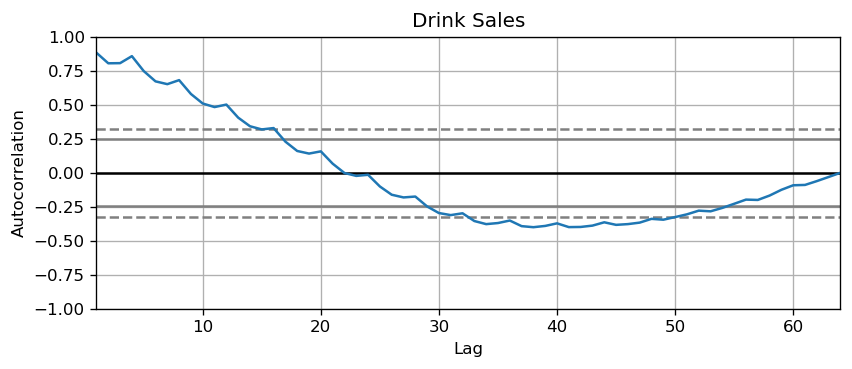
The common way is to plot the series and check for repeatable patterns in fixed time intervals. However, if you want a more definitive inspection of the seasonality, use the Autocorrelation Function (ACF) plot. Strong patterns in real word datasets is hardly noticed and can get distorted by any noise, so you need a careful eye to capture these patterns.
Alternately, if you want a statistical test, the Canova-Hansen test for seasonal differences can determine if seasonal differencing is required to stationarize the series.
[44]:
plot_autocorr(df_house.sales,'House Sales')
[45]:
plot_autocorr(df_drink.sales,'Drink Sales')
Missing Values in a Time Series
When the time series have missing dates or times, the data was not captured or available for those periods. We may need to fill up those periods with a reasonable value. It is typically not a good idea to replace missing values with the mean of the series, especially if the series is not stationary.
Depending on the nature of the series, there are a few approaches are available:
Forward Fill
Backward Fill
Linear Interpolation
Quadratic interpolation
Mean of nearest neighbors
Mean of seasonal couterparts
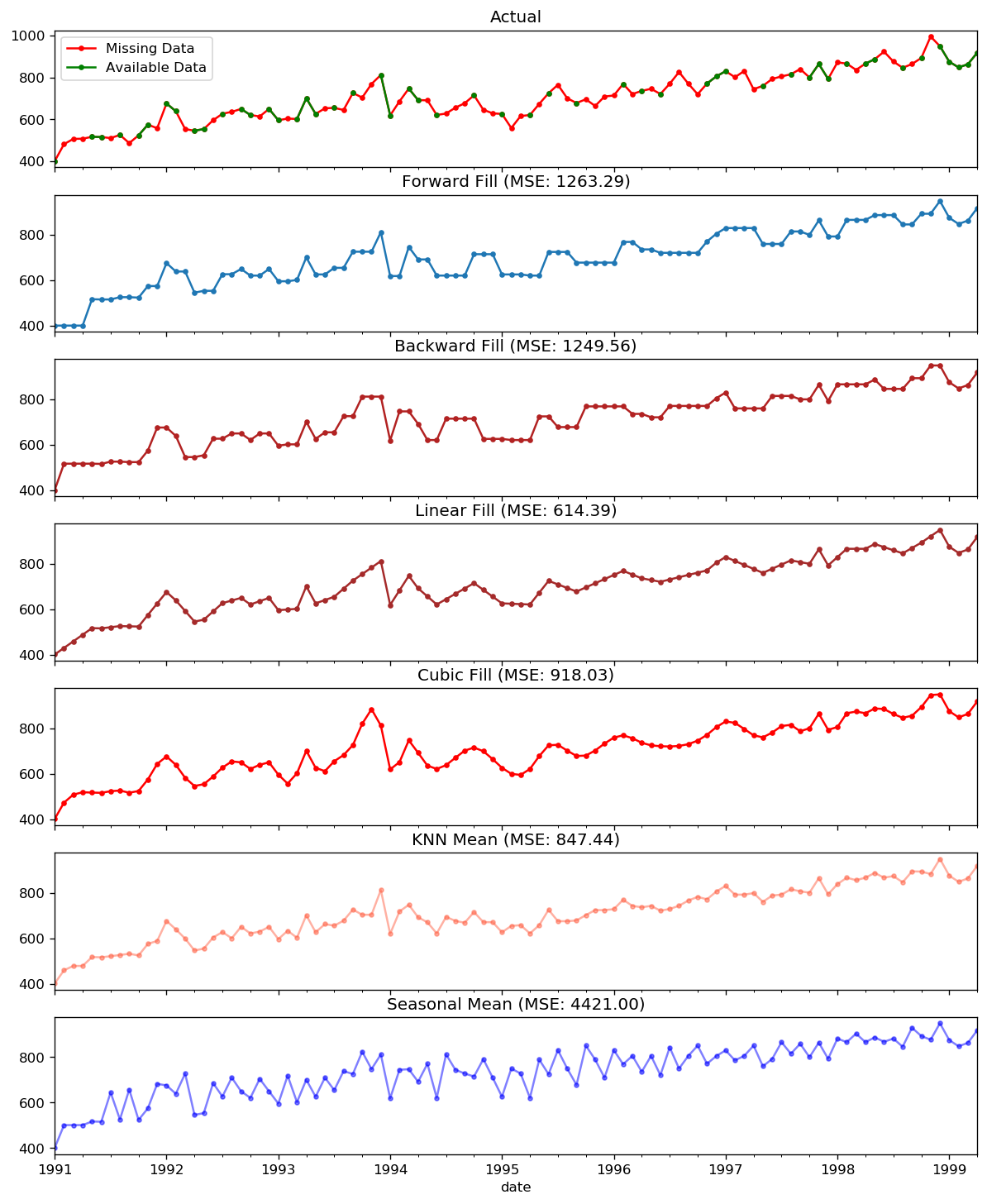
In the demonstration, we manually introduce missing values to the time series and impute it with above approaches. Since the original non-missing values are known, we can measure the imputation performance by calculating the mean squared error (MSE) of the imputed against the actual values.
More interesting approaches can be considered:
If explanatory variables are available, we can use a prediction model such as the random forest or k-Nearest Neighbors to predict missing values.
If past observations are enough, we can forecast the missing values.
If future observations are enough, we can backcast the missing values
We can also forecast the counterparts from previous cycles.
[46]:
from scipy.interpolate import interp1d
from sklearn.metrics import mean_squared_error

dataurl = 'https://raw.githubusercontent.com/ming-zhao/Business-Analytics/master/data/time_series/'

# for easy demonstration, we only consider 100 observations
df_orig = pd.read_csv(dataurl+'house_sales.csv', parse_dates=['date'], index_col='date').head(100)

df_missing = pd.read_csv(dataurl+'house_sales_missing.csv', parse_dates=['date'], index_col='date')

fig, axes = plt.subplots(7, 1, sharex=True, figsize=(12, 15))
plt.rcParams.update({'xtick.bottom' : False})

## 1. Actual -------------------------------
df_orig.plot(y="sales", title='Actual', ax=axes[0], label='Actual', color='red', style=".-")
df_missing.plot(y="sales", title='Actual', ax=axes[0], label='Actual', color='green', style=".-")
axes[0].legend(["Missing Data", "Available Data"])

## 2. Forward Fill --------------------------
df_ffill = df_missing.ffill()
error = np.round(mean_squared_error(df_orig['sales'], df_ffill['sales']), 2)
df_ffill['sales'].plot(title='Forward Fill (MSE: ' + str(error) +")",
                             ax=axes[1], label='Forward Fill', style=".-")
## 3. Backward Fill -------------------------
df_bfill = df_missing.bfill()
error = np.round(mean_squared_error(df_orig['sales'], df_bfill['sales']), 2)
df_bfill['sales'].plot(title="Backward Fill (MSE: " + str(error) +")",
                             ax=axes[2], label='Back Fill', color='firebrick', style=".-")

## 4. Linear Interpolation ------------------
df_missing['rownum'] = np.arange(df_missing.shape[0])
df_nona = df_missing.dropna(subset = ['sales'])
f = interp1d(df_nona['rownum'], df_nona['sales'])
df_missing['linear_fill'] = f(df_missing['rownum'])
error = np.round(mean_squared_error(df_orig['sales'], df_missing['linear_fill']), 2)
df_missing['linear_fill'].plot(title="Linear Fill (MSE: " + str(error) +")",
                       ax=axes[3], label='Cubic Fill', color='brown', style=".-")

## 5. Cubic Interpolation --------------------
f2 = interp1d(df_nona['rownum'], df_nona['sales'], kind='cubic')
df_missing['cubic_fill'] = f2(df_missing['rownum'])
error = np.round(mean_squared_error(df_orig['sales'], df_missing['cubic_fill']), 2)
df_missing['cubic_fill'].plot(title="Cubic Fill (MSE: " + str(error) +")",
                              ax=axes[4], label='Cubic Fill', color='red', style=".-")

# Interpolation References:
# https://docs.scipy.org/doc/scipy/reference/tutorial/interpolate.html
# https://docs.scipy.org/doc/scipy/reference/interpolate.html

## 6. Mean of 'n' Nearest Past Neighbors ------
def knn_mean(ts, n):
    out = np.copy(ts)
    for i, val in enumerate(ts):
        if np.isnan(val):
            n_by_2 = np.ceil(n/2)
            lower = np.max([0, int(i-n_by_2)])
            upper = np.min([len(ts)+1, int(i+n_by_2)])
            ts_near = np.concatenate([ts[lower:i], ts[i:upper]])
            out[i] = np.nanmean(ts_near)
    return out

df_missing['knn_mean'] = knn_mean(df_missing['sales'].values, 8)
error = np.round(mean_squared_error(df_orig['sales'], df_missing['knn_mean']), 2)
df_missing['knn_mean'].plot(title="KNN Mean (MSE: " + str(error) +")",
                            ax=axes[5], label='KNN Mean', color='tomato', alpha=0.5, style=".-")

# 7. Seasonal Mean ----------------------------
def seasonal_mean(ts, n, lr=0.7):
    """
    Compute the mean of corresponding seasonal periods
    ts: 1D array-like of the time series
    n: Seasonal window length of the time series
    """
    out = np.copy(ts)
    for i, val in enumerate(ts):
        if np.isnan(val):
            ts_seas = ts[i-1::-n]  # previous seasons only
            out[i] = out[i-1]
            if ~ts_seas.isnull().all():
                if np.isnan(np.nanmean(ts_seas)):
                    ts_seas = np.concatenate([ts[i-1::-n], ts[i::n]])  # previous and forward
                out[i] = np.nanmean(ts_seas) * lr
    return out

df_missing['seasonal_mean'] = seasonal_mean(df_missing['sales'], n=6, lr=1.25)
error = np.round(mean_squared_error(df_orig['sales'], df_missing['seasonal_mean']), 2)
df_missing['seasonal_mean'].plot(title="Seasonal Mean (MSE: {:.2f})".format(error),
                         ax=axes[6], label='Seasonal Mean', color='blue', alpha=0.5, style=".-")
plt.show()
toggle()
[46]:
Autocorrelation and Partial Autocorrelation
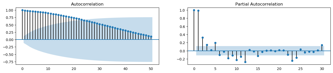
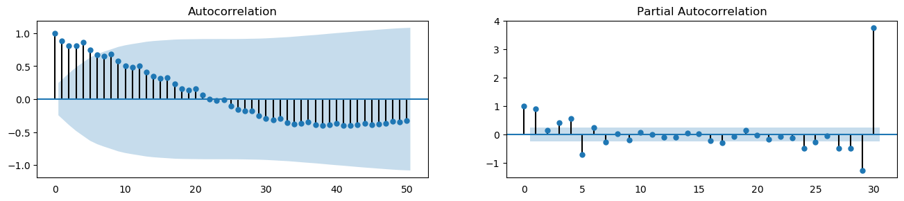
We can calculate the correlation for time series observations with observations in previous time steps, called lags. Because the correlation of the time series observations is calculated with values of the same series at previous times, this is called a serial correlation, or an autocorrelation. If a series is significantly autocorrelated, then the previous values of the series (lags) may be helpful in predicting the current value.
A partial autocorrelation is a summary of the relationship between an observation in a time series with observations at prior time steps with the relationships of intervening observations removed (i.e., excluding the correlation contributions from the intermediate lags). The partial autocorrelation at lag \(k\) is the correlation that results after removing the effect of any correlations due to the terms at shorter lags.
The partial autocorrelation of lag (k) of a series is the coefficient of that lag in the autoregression equation of Y. The autoregressive equation of Y is nothing but the linear regression of Y with its own lags as predictors. For example, let \(Y_t\) be the current value, then the partial autocorrelation of lag 3 (\(Y_{t-3}\)) is the coefficient \(\alpha_3\) in the following equation:
[47]:
plot_acf_pacf(df_house.sales, 50, 30)
[48]:
plot_acf_pacf(df_drink.sales, 50, 30)
A Lag plot is a scatter plot of a time series against a lag of itself. It is normally used to check for autocorrelation. If there is any pattern existing in the series (such as house sales with lag 1 and drink sales with lag 4), the series is autocorrelated. If there is no pattern, the series is likely to be random white noise.
As shown in the figures, points get wide and scattered with increasing lag which indicates lesser correlation.
[49]:
interact(house_drink_lag,
         house_lag=widgets.IntSlider(min=1,max=43,step=3,value=1,description='House Lag:'),
         drink_lag=widgets.IntSlider(min=1,max=43,step=3,value=1,description='Drink Lag:'));

interact(noise_rndwalk_lag,
         noise_lag=widgets.IntSlider(min=1,max=43,step=3,value=1,description='White Noise Lag:',
                                    style = {'description_width': 'initial'}),
         rndwalk_lag=widgets.IntSlider(min=1,max=43,step=3,value=1,description='Random Walk Lag:',
                                      style = {'description_width': 'initial'}));
ARIMA Models
ARIMA is an acronym that stands for AutoRegressive Integrated Moving Average. It is a forecasting algorithm based on the idea that the information in the past values of the time series (i.e. its own lags and the lagged forecast errors) can alone be used to predict the future values.
Any non-seasonal time series that exhibits patterns and is not a random white noise can be modeled with ARIMA models.
The acronym ARIMA is descriptive, capturing the key aspects of the model itself. Briefly, they are:
AR: Autoregression. A model that uses the dependent relationship between an observation and some number of lagged observations. An autoregressive model of order \(p\) (AR(p)) can be written as
I: Integrated. The use of differencing of raw observations (e.g. subtracting an observation from an observation at the previous time step) in order to make the time series stationary.
MA: Moving Average. A model that uses the dependency between an observation and a residual error from a moving average model applied to lagged observations. An moving average model of order \(q\) (MA(q)) can be written as
Each of these components are explicitly specified in the model as a parameter. A standard notation is used of ARIMA(p,d,q) where the parameters are substituted with integer values to quickly indicate the specific ARIMA model being used. The parameters of the ARIMA model are defined as follows:
\(d\) is the number of differencing required to make the time series stationary
\(p\) is the number of lag observations included in the model, i.e., the order of the AR term
\(q\) is The size of the moving average window, i.e., the order of the MA term
The ARIMA(p,d,q) model can be written as
\begin{equation} Y^\prime_{t} = c + \phi_{1}Y^\prime_{t-1} + \cdots + \phi_{p}Y^\prime_{t-p} + \theta_{1}e_{t-1} + \cdots + \theta_{q}e_{t-q} + e_{t}, \end{equation}
where \(Y^\prime_{t}\) is the differenced series (it may have been differenced more than once). The ARIMA\((p,d,q)\) model in words:
predicted \(Y_t\) = Constant + Linear combination Lags of \(Y\) (upto \(p\) lags) + Linear Combination of Lagged forecast errors (upto \(q\) lags)
The objective, therefore, is to identify the values of p, d and q. A value of 0 can be used for a parameter, which indicates to not use that element of the model. This way, the ARIMA model can be configured to perform the function of an ARMA model, and even a simple AR, I, or MA model.
How to make a series stationary?
The most common approach is to difference it. That is, subtract the previous value from the current value. Sometimes, depending on the complexity of the series, more than one differencing may be needed.
The value of \(d\), therefore, is the minimum number of differencing needed to make the series stationary. And if the time series is already stationary, then \(d = 0\).
Why make the time series stationary?
Because, term “Auto Regressive” in ARIMA means it is a linear regression model that uses its own lags as predictors. Linear regression models work best when the predictors are not correlated and are independent of each other. So we take differences to remove trend and seasonal structures that negatively affect the regression model.
Identify the Order of Differencing
The right order of differencing is the minimum differencing required to get a near-stationary series which roams around a defined mean and the ACF plot reaches to zero fairly quick. If the autocorrelations are positive for many number of lags (10 or more), then the series needs further differencing. On the other hand, if the lag 1 autocorrelation itself is too negative, then the series is probably over-differenced. If we can’t really decide between different orders of differencing, then go with the order that gives the least standard deviation in the differenced series.
[50]:
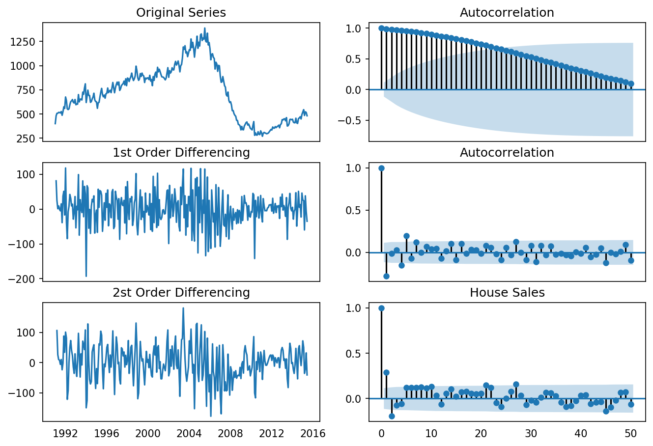
differencing(df_house, 'sales', title='House Sales')
Standard deviation original series: 279.720
Standard deviation 1st differencing: 48.344
Standard deviation 2st differencing: 57.802
[51]:
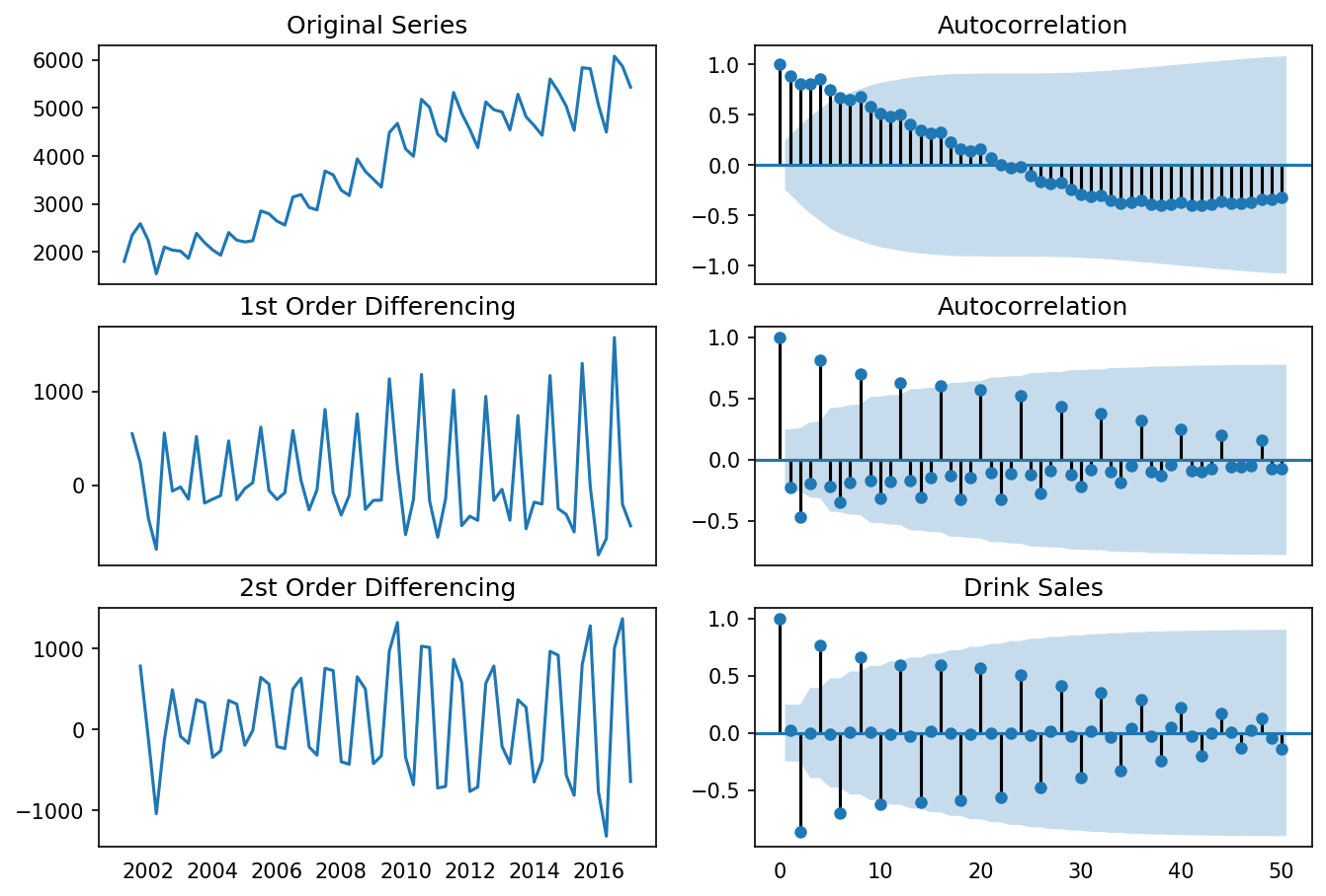
differencing(df_drink, 'sales', title='Drink Sales')
Standard deviation original series: 1283.446
Standard deviation 1st differencing: 532.296
Standard deviation 2st differencing: 661.759
Recall that ADF test shows that the house sales data is not stationary. On looking at the autocorrelation plot for the first differencing the lag goes into the negative zone, which indicates that the series might have been over differenced. We tentatively fix the order of differencing as \(d=1\) even though the series is a bit overdifferenced.
Identify the Order of the MA and AR Terms
If the ACF of the differenced series displays a sharp cutoff and/or the lag-1 autocorrelation is negative - i.e., if the series appears slightly “overdifferenced” - then consider adding an MA term to the model. The lag at which the ACF cuts off is the indicated number of MA terms.
If the PACF of the differenced series displays a sharp cutoff and/or the lag-1 autocorrelation is positive - i.e., if the series appears slightly “underdifferenced” - then consider adding an AR term to the model. The lag at which the PACF cuts off is the indicated number of AR terms.
[52]:
from statsmodels.graphics.tsaplots import plot_acf, plot_pacf
plt.rcParams.update({'figure.figsize':(9,3), 'figure.dpi':120})
fig, axes = plt.subplots(1, 2)
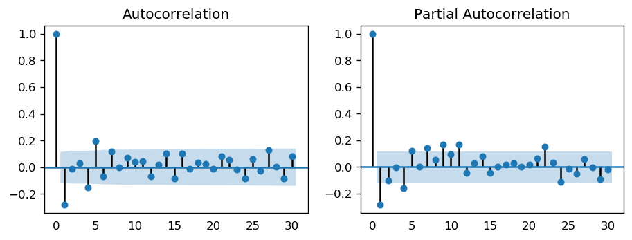
plot_acf(df_house.sales.diff().dropna(), lags=30, ax=axes[0])
plot_pacf(df_house.sales.diff().dropna(), lags=30, ax=axes[1])
plt.show()
toggle()
[52]:
The single negative spike at lag 1 in the ACF is an MA(1) signature, according to rule above. Thus, if we were to use 1 nonseasonal differences, we would also want to include an MA(1) term, yielding an ARIMA(0,1,1) model.
In most cases, the best model turns out a model that uses either only AR terms or only MA terms, although in some cases a “mixed” model with both AR and MA terms may provide the best fit to the data. However, care must be exercised when fitting mixed models. It is possible for an AR term and an MA term to cancel each other’s effects, even though both may appear significant in the model (as judged by the t-statistics of their coefficients).
[53]:
widgets.interact_manual.opts['manual_name'] = 'Run ARIMA'
interact_manual(arima_,
         p=widgets.BoundedIntText(value=0, min=0, step=1, description='p:', disabled=False),
         d=widgets.BoundedIntText(value=1, min=0, max=2, step=1, description='d:', disabled=False),
         q=widgets.BoundedIntText(value=1, min=0, step=1, description='q:', disabled=False));

arima_(0, 1, 1)
| Dep. Variable: | D.sales | No. Observations: | 293 |
|---|---|---|---|
| Model: | ARIMA(0, 1, 1) | Log Likelihood | -1538.134 |
| Method: | css-mle | S.D. of innovations | 46.084 |
| Date: | Thu, 22 Aug 2019 | AIC | 3082.268 |
| Time: | 10:02:55 | BIC | 3093.308 |
| Sample: | 02-01-1991 | HQIC | 3086.690 |
| - 06-01-2015 |
| coef | std err | z | P>|z| | [0.025 | 0.975] | |
|---|---|---|---|---|---|---|
| const | 0.2164 | 1.823 | 0.119 | 0.906 | -3.356 | 3.789 |
| ma.L1.D.sales | -0.3241 | 0.057 | -5.724 | 0.000 | -0.435 | -0.213 |
| Real | Imaginary | Modulus | Frequency | |
|---|---|---|---|---|
| MA.1 | 3.0859 | +0.0000j | 3.0859 | 0.0000 |
The table in the middle is the coefficients table where the values under coef are the weights of the respective terms. Ideally, we expect to have the P-Value in P>|z| column is less than 0.05 for the respective coef to be significant.
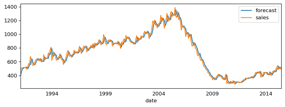
The setting dynamic=False in plot_predict uses the in-sample lagged values for prediction. The model gets trained up until the previous value to make the next prediction. This setting can make the fitted forecast and actuals look artificially good. Hence, we seem to have a decent ARIMA model. But is that the best? Can’t say that at this point because we haven’t actually forecasted into the future and compared the forecast with the actual performance. The real validation you need now is
the Out-of-Sample cross-validation.
Identify the Optimal ARIMA Model
We create the training and testing datasets by splitting the time series into two contiguous parts in approximately 75:25 ratio or a reasonable proportion based on time frequency of series.
[54]:
widgets.interact_manual.opts['manual_name'] = 'Run ARIMA'
interact_manual(arima_validation,
         p=widgets.BoundedIntText(value=0, min=0, step=1, description='p:', disabled=False),
         d=widgets.BoundedIntText(value=1, min=0, max=2, step=1, description='d:', disabled=False),
         q=widgets.BoundedIntText(value=1, min=0, step=1, description='q:', disabled=False));

arima_validation(0, 1, 1)
| Dep. Variable: | D.sales | No. Observations: | 220 |
|---|---|---|---|
| Model: | ARIMA(0, 1, 1) | Log Likelihood | -1174.593 |
| Method: | css-mle | S.D. of innovations | 50.394 |
| Date: | Thu, 22 Aug 2019 | AIC | 2355.186 |
| Time: | 10:02:56 | BIC | 2365.367 |
| Sample: | 02-01-1991 | HQIC | 2359.297 |
| - 05-01-2009 |
| coef | std err | z | P>|z| | [0.025 | 0.975] | |
|---|---|---|---|---|---|---|
| const | -0.2968 | 2.316 | -0.128 | 0.898 | -4.835 | 4.242 |
| ma.L1.D.sales | -0.3200 | 0.065 | -4.936 | 0.000 | -0.447 | -0.193 |
| Real | Imaginary | Modulus | Frequency | |
|---|---|---|---|---|
| MA.1 | 3.1249 | +0.0000j | 3.1249 | 0.0000 |
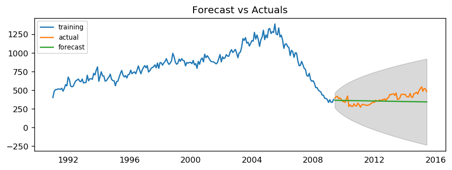
MAPE : 0.1626
The model seems to give a directionally correct forecast and the actual observed values lie within the 95% confidence band.
A much more convenient approach is to use auto_arima() which searches multiple combinations of \(p,d,q\) parameters and chooses the best model. see auto_arima() manual for parameters settings.
[55]:
from statsmodels.tsa.arima_model import ARIMA

arima_house = pm.auto_arima(df_house.sales,
                      start_p=0, start_q=0,
                      test='adf',       # use adftest to find optimal 'd'
                      max_p=4, max_q=4, # maximum p and q
                      m=12,             # 12 for monthly data
                      d=None,           # let model determine 'd' differencing
                      seasonal=False,   # No Seasonality
                      #start_P=0,       # order of the auto-regressive portion of the seasonal model
                      #D=0,             # order of the seasonal differencing
                      #start_Q=0,       # order of the moving-average portion of the seasonal model
                      trace=True,
                      error_action='ignore',
                      suppress_warnings=True,
                      stepwise=True)

display(arima_house.summary())
_ = arima_house.plot_diagnostics(figsize=(10,7));
toggle()
Fit ARIMA: order=(0, 1, 0); AIC=3108.202, BIC=3115.562, Fit time=0.002 seconds
Fit ARIMA: order=(1, 1, 0); AIC=3085.720, BIC=3096.761, Fit time=0.036 seconds
Fit ARIMA: order=(0, 1, 1); AIC=3082.268, BIC=3093.308, Fit time=0.039 seconds
Fit ARIMA: order=(1, 1, 1); AIC=3084.181, BIC=3098.901, Fit time=0.067 seconds
Fit ARIMA: order=(0, 1, 2); AIC=3084.182, BIC=3098.903, Fit time=0.065 seconds
Fit ARIMA: order=(1, 1, 2); AIC=3086.179, BIC=3104.580, Fit time=0.110 seconds
Total fit time: 0.330 seconds
| Dep. Variable: | D.y | No. Observations: | 293 |
|---|---|---|---|
| Model: | ARIMA(0, 1, 1) | Log Likelihood | -1538.134 |
| Method: | css-mle | S.D. of innovations | 46.084 |
| Date: | Thu, 22 Aug 2019 | AIC | 3082.268 |
| Time: | 10:02:57 | BIC | 3093.308 |
| Sample: | 1 | HQIC | 3086.690 |
| coef | std err | z | P>|z| | [0.025 | 0.975] | |
|---|---|---|---|---|---|---|
| const | 0.2164 | 1.823 | 0.119 | 0.906 | -3.356 | 3.789 |
| ma.L1.D.y | -0.3241 | 0.057 | -5.724 | 0.000 | -0.435 | -0.213 |
| Real | Imaginary | Modulus | Frequency | |
|---|---|---|---|---|
| MA.1 | 3.0859 | +0.0000j | 3.0859 | 0.0000 |
[55]:
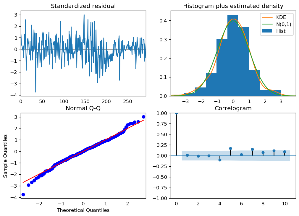
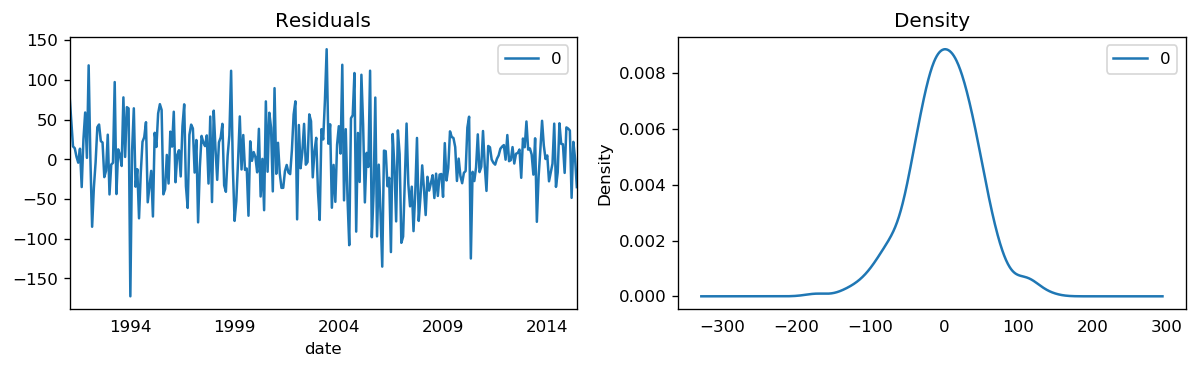
We can review the residual plots.
Standardized resitual: The residual errors seem to fluctuate around a mean of zero and have a uniform variance.
Histogram plus estimated density: The density plot suggests normal distribution with mean zero.
Normal Q-Q: All the dots should fall perfectly in line with the red line. Any significant deviations would imply the distribution is skewed.
Correlogram: The Correlogram (ACF plot) shows the residual errors are not autocorrelated. Any autocorrelation would imply that there is some pattern in the residual errors which are not explained in the model.
ARIMA forecast
[56]:
# Forecast
n_periods = 24
fc, conf = arima_house.predict(n_periods=n_periods, return_conf_int=True)
index_of_fc = pd.period_range(df_house.index[-1], freq='M', periods=n_periods+1)[1:].astype('datetime64[ns]')

# make series for plotting purpose
fc_series = pd.Series(fc, index=index_of_fc)
lower_series = pd.Series(conf[:, 0], index=index_of_fc)
upper_series = pd.Series(conf[:, 1], index=index_of_fc)

# Plot
plt.plot(df_house.sales)
plt.plot(fc_series, color='darkgreen')
plt.fill_between(lower_series.index,
                 lower_series,
                 upper_series,
                 color='k', alpha=.15)

plt.title("Final Forecast of House Sales")
plt.show()

toggle()
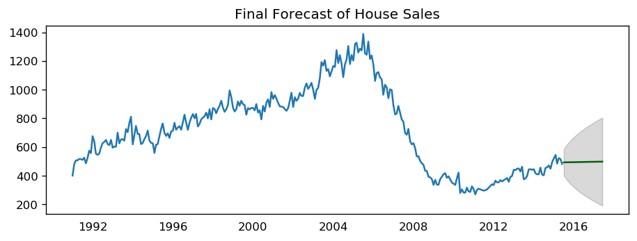
[56]:
ARIMA vs Exponential Smoothing Models
While linear exponential smoothing models are all special cases of ARIMA models, the non-linear exponential smoothing models have no equivalent ARIMA counterparts. On the other hand, there are also many ARIMA models that have no exponential smoothing counterparts. In particular, all exponential smoothing models are non-stationary, while some ARIMA models are stationary.
Seasonal ARIMA (SARIMA) Models
The ARIMA model does not support seasonality. If the time series data has defined seasonality, then we need to perform seasonal differencing and SARIMA models.
Seasonal differencing is similar to regular differencing, but, instead of subtracting consecutive terms, we subtract the value from previous season.
The model is represented as SARIMA\((p,d,q)x(P,D,Q)\), where - \(D\) is the order of seasonal differencing - \(P\) is the order of seasonal autoregression (SAR) - \(Q\) is the order of seasonal moving average (SMA) - \(x\) is the frequency of the time series.
[57]:
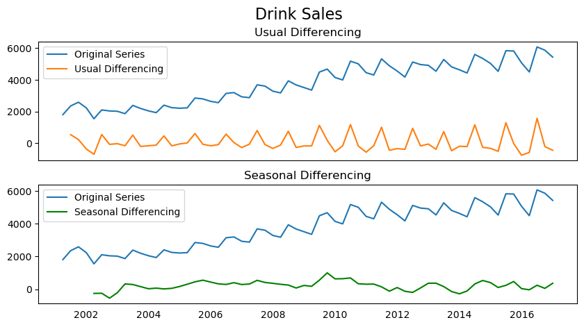
fig, axes = plt.subplots(2, 1, figsize=(10,5), dpi=100, sharex=True)

# Usual Differencing
axes[0].plot(df_drink.sales, label='Original Series')
axes[0].plot(df_drink.sales.diff(1), label='Usual Differencing')
axes[0].set_title('Usual Differencing')
axes[0].legend(loc='upper left', fontsize=10)


# Seasinal Differencing
axes[1].plot(df_drink.sales, label='Original Series')
axes[1].plot(df_drink.sales.diff(4), label='Seasonal Differencing', color='green')
axes[1].set_title('Seasonal Differencing')
plt.legend(loc='upper left', fontsize=10)
plt.suptitle('Drink Sales', fontsize=16)
plt.show()

toggle()
[57]:
As we can clearly see, the seasonal spikes is intact after applying usual differencing (lag 1). Whereas, it is rectified after seasonal differencing.
Find optimal SARIMA for house sales:
[58]:
sarima_house = pm.auto_arima(df_house.sales,
                       start_p=1, start_q=1,
                       test='adf',
                       max_p=3, max_q=3, m=4,
                       start_P=0, seasonal=True,
                       d=None, D=1, trace=True,
                       error_action='ignore',
                       suppress_warnings=True,
                       stepwise=True)

sarima_house.summary()
Fit ARIMA: order=(1, 0, 1) seasonal_order=(0, 1, 1, 4); AIC=3069.410, BIC=3087.760, Fit time=0.459 seconds
Fit ARIMA: order=(0, 0, 0) seasonal_order=(0, 1, 0, 4); AIC=3317.294, BIC=3324.633, Fit time=0.014 seconds
Fit ARIMA: order=(1, 0, 0) seasonal_order=(1, 1, 0, 4); AIC=3167.461, BIC=3182.141, Fit time=0.279 seconds
Fit ARIMA: order=(0, 0, 1) seasonal_order=(0, 1, 1, 4); AIC=3242.302, BIC=3256.981, Fit time=0.268 seconds
Fit ARIMA: order=(1, 0, 1) seasonal_order=(1, 1, 1, 4); AIC=3068.583, BIC=3090.603, Fit time=0.600 seconds
Fit ARIMA: order=(1, 0, 1) seasonal_order=(1, 1, 0, 4); AIC=3144.929, BIC=3163.278, Fit time=0.454 seconds
Fit ARIMA: order=(1, 0, 1) seasonal_order=(1, 1, 2, 4); AIC=3068.574, BIC=3094.263, Fit time=1.156 seconds
Fit ARIMA: order=(0, 0, 1) seasonal_order=(1, 1, 2, 4); AIC=3212.955, BIC=3234.974, Fit time=0.574 seconds
Fit ARIMA: order=(2, 0, 1) seasonal_order=(1, 1, 2, 4); AIC=3070.429, BIC=3099.788, Fit time=1.276 seconds
Fit ARIMA: order=(1, 0, 0) seasonal_order=(1, 1, 2, 4); AIC=3092.690, BIC=3114.709, Fit time=1.139 seconds
Fit ARIMA: order=(1, 0, 2) seasonal_order=(1, 1, 2, 4); AIC=3075.044, BIC=3104.403, Fit time=1.402 seconds
Fit ARIMA: order=(0, 0, 0) seasonal_order=(1, 1, 2, 4); AIC=3275.870, BIC=3294.219, Fit time=0.476 seconds
Fit ARIMA: order=(2, 0, 2) seasonal_order=(1, 1, 2, 4); AIC=3067.394, BIC=3100.423, Fit time=2.353 seconds
Fit ARIMA: order=(2, 0, 2) seasonal_order=(0, 1, 2, 4); AIC=3067.596, BIC=3096.955, Fit time=2.287 seconds
Fit ARIMA: order=(2, 0, 2) seasonal_order=(2, 1, 2, 4); AIC=3075.797, BIC=3112.496, Fit time=2.674 seconds
Fit ARIMA: order=(2, 0, 2) seasonal_order=(1, 1, 1, 4); AIC=3071.372, BIC=3100.731, Fit time=1.910 seconds
Fit ARIMA: order=(2, 0, 2) seasonal_order=(0, 1, 1, 4); AIC=3066.271, BIC=3091.960, Fit time=1.455 seconds
Fit ARIMA: order=(1, 0, 2) seasonal_order=(0, 1, 1, 4); AIC=3071.461, BIC=3093.481, Fit time=0.649 seconds
Fit ARIMA: order=(3, 0, 2) seasonal_order=(0, 1, 1, 4); AIC=3088.496, BIC=3117.855, Fit time=1.228 seconds
Fit ARIMA: order=(2, 0, 1) seasonal_order=(0, 1, 1, 4); AIC=3071.301, BIC=3093.320, Fit time=0.548 seconds
Fit ARIMA: order=(2, 0, 3) seasonal_order=(0, 1, 1, 4); AIC=3071.104, BIC=3100.463, Fit time=0.785 seconds
Fit ARIMA: order=(3, 0, 3) seasonal_order=(0, 1, 1, 4); AIC=3073.092, BIC=3106.121, Fit time=0.942 seconds
Fit ARIMA: order=(2, 0, 2) seasonal_order=(0, 1, 0, 4); AIC=3195.762, BIC=3217.781, Fit time=0.642 seconds
Total fit time: 23.584 seconds
[58]:
| Dep. Variable: | y | No. Observations: | 294 |
|---|---|---|---|
| Model: | SARIMAX(2, 0, 2)x(0, 1, 1, 4) | Log Likelihood | -1526.135 |
| Date: | Thu, 22 Aug 2019 | AIC | 3066.271 |
| Time: | 10:03:23 | BIC | 3091.960 |
| Sample: | 0 | HQIC | 3076.563 |
| - 294 | |||
| Covariance Type: | opg |
| coef | std err | z | P>|z| | [0.025 | 0.975] | |
|---|---|---|---|---|---|---|
| intercept | 0.0041 | 0.068 | 0.060 | 0.952 | -0.129 | 0.137 |
| ar.L1 | 0.1825 | 0.116 | 1.575 | 0.115 | -0.045 | 0.410 |
| ar.L2 | 0.8102 | 0.091 | 8.931 | 0.000 | 0.632 | 0.988 |
| ma.L1 | 0.5482 | 0.118 | 4.664 | 0.000 | 0.318 | 0.779 |
| ma.L2 | -0.3360 | 0.057 | -5.890 | 0.000 | -0.448 | -0.224 |
| ma.S.L4 | -0.9908 | 0.151 | -6.549 | 0.000 | -1.287 | -0.694 |
| sigma2 | 2078.7585 | 281.748 | 7.378 | 0.000 | 1526.543 | 2630.975 |
| Ljung-Box (Q): | 64.52 | Jarque-Bera (JB): | 5.87 |
|---|---|---|---|
| Prob(Q): | 0.01 | Prob(JB): | 0.05 |
| Heteroskedasticity (H): | 0.50 | Skew: | -0.05 |
| Prob(H) (two-sided): | 0.00 | Kurtosis: | 3.69 |
Warnings:
[1] Covariance matrix calculated using the outer product of gradients (complex-step).
Find optimal SARIMA for drink sales
[59]:
sarima_drink = pm.auto_arima(df_drink.sales,
                       start_p=1, start_q=1,
                       test='adf',
                       max_p=3, max_q=3, m=4,
                       start_P=0, seasonal=True,
                       d=None, D=1, trace=True,
                       error_action='ignore',
                       suppress_warnings=True,
                       stepwise=True)

sarima_drink.summary()
Fit ARIMA: order=(1, 0, 1) seasonal_order=(0, 1, 1, 4); AIC=809.758, BIC=820.230, Fit time=0.133 seconds
Fit ARIMA: order=(0, 0, 0) seasonal_order=(0, 1, 0, 4); AIC=848.072, BIC=852.261, Fit time=0.006 seconds
Fit ARIMA: order=(1, 0, 0) seasonal_order=(1, 1, 0, 4); AIC=813.870, BIC=822.248, Fit time=0.042 seconds
Fit ARIMA: order=(0, 0, 1) seasonal_order=(0, 1, 1, 4); AIC=813.808, BIC=822.185, Fit time=0.129 seconds
Fit ARIMA: order=(1, 0, 1) seasonal_order=(1, 1, 1, 4); AIC=811.609, BIC=824.175, Fit time=0.166 seconds
Fit ARIMA: order=(1, 0, 1) seasonal_order=(0, 1, 0, 4); AIC=810.383, BIC=818.760, Fit time=0.104 seconds
Fit ARIMA: order=(1, 0, 1) seasonal_order=(0, 1, 2, 4); AIC=811.498, BIC=824.064, Fit time=0.183 seconds
Fit ARIMA: order=(1, 0, 1) seasonal_order=(1, 1, 2, 4); AIC=813.470, BIC=828.130, Fit time=0.246 seconds
Fit ARIMA: order=(2, 0, 1) seasonal_order=(0, 1, 1, 4); AIC=811.201, BIC=823.767, Fit time=0.281 seconds
Fit ARIMA: order=(1, 0, 0) seasonal_order=(0, 1, 1, 4); AIC=813.022, BIC=821.399, Fit time=0.113 seconds
Fit ARIMA: order=(1, 0, 2) seasonal_order=(0, 1, 1, 4); AIC=810.926, BIC=823.492, Fit time=0.351 seconds
Fit ARIMA: order=(0, 0, 0) seasonal_order=(0, 1, 1, 4); AIC=849.704, BIC=855.987, Fit time=0.054 seconds
Fit ARIMA: order=(2, 0, 2) seasonal_order=(0, 1, 1, 4); AIC=813.065, BIC=827.725, Fit time=0.304 seconds
Total fit time: 2.121 seconds
[59]:
| Dep. Variable: | y | No. Observations: | 64 |
|---|---|---|---|
| Model: | SARIMAX(1, 0, 1)x(0, 1, 1, 4) | Log Likelihood | -399.879 |
| Date: | Thu, 22 Aug 2019 | AIC | 809.758 |
| Time: | 10:03:25 | BIC | 820.230 |
| Sample: | 0 | HQIC | 813.854 |
| - 64 | |||
| Covariance Type: | opg |
| coef | std err | z | P>|z| | [0.025 | 0.975] | |
|---|---|---|---|---|---|---|
| intercept | 121.9284 | 50.994 | 2.391 | 0.017 | 21.981 | 221.876 |
| ar.L1 | 0.4436 | 0.178 | 2.492 | 0.013 | 0.095 | 0.793 |
| ma.L1 | 0.5287 | 0.143 | 3.687 | 0.000 | 0.248 | 0.810 |
| ma.S.L4 | -0.2772 | 0.141 | -1.969 | 0.049 | -0.553 | -0.001 |
| sigma2 | 3.487e+04 | 6857.056 | 5.085 | 0.000 | 2.14e+04 | 4.83e+04 |
| Ljung-Box (Q): | 28.74 | Jarque-Bera (JB): | 0.83 |
|---|---|---|---|
| Prob(Q): | 0.91 | Prob(JB): | 0.66 |
| Heteroskedasticity (H): | 1.28 | Skew: | -0.29 |
| Prob(H) (two-sided): | 0.58 | Kurtosis: | 3.03 |
Warnings:
[1] Covariance matrix calculated using the outer product of gradients (complex-step).
We perform forecasting using SARIMA
[60]:
sarima_forcast(sarima_house, df_house, 'sales', forecast_periods=24, freq='month')
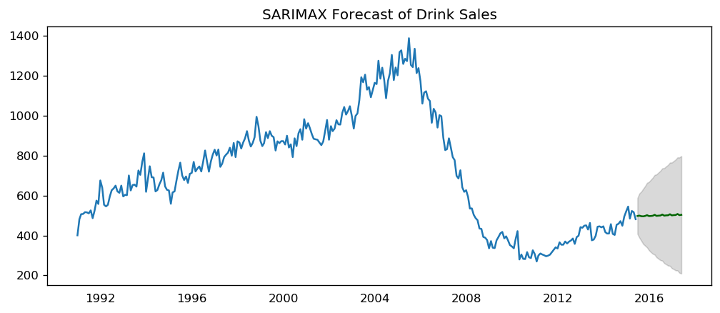
[61]:
sarima_forcast(sarima_drink, df_drink, 'sales', forecast_periods=24, freq='quarter')
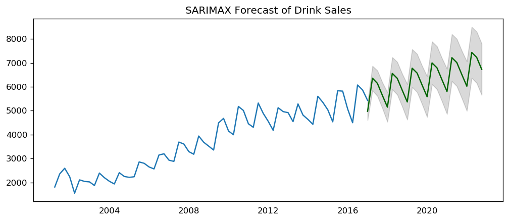
SARIMAX Model with Exogenous Variable
We have a SARIMA model if there is an external predictor, also called, “exogenous variable” built into SARIMA models. The only requirement to use an exogenous variable is that we need to know the value of the variable during the forecast period as well.
For the sake of demonstration, we use the seasonal index from the classical seasonal decomposition on the latest 3 years of data even though SARIMA already modeling the seasonality.
The seasonal index is a good exogenous variable for demonstration purpose because it repeats every frequency cycle, 4 quarters in this case. So, we always know what values the seasonal index will hold for the future forecasts.
[62]:
df_drink = add_seasonal_index(df_drink, 'sales', freq='quarter', model='multiplicative')
sarimax_drink = pm.auto_arima(df_drink[['sales']], exogenous=df_drink[['seasonal_index']],
                           start_p=1, start_q=1,
                           test='adf',
                           max_p=3, max_q=3, m=12,
                           start_P=0, seasonal=True,
                           d=None, D=1, trace=True,
                           error_action='ignore',
                           suppress_warnings=True,
                           stepwise=True)

sarimax_drink.summary()
Fit ARIMA: order=(1, 1, 1) seasonal_order=(0, 1, 1, 12); AIC=727.512, BIC=739.103, Fit time=0.645 seconds
Fit ARIMA: order=(0, 1, 0) seasonal_order=(0, 1, 0, 12); AIC=730.208, BIC=736.003, Fit time=0.011 seconds
Fit ARIMA: order=(1, 1, 0) seasonal_order=(1, 1, 0, 12); AIC=726.724, BIC=736.383, Fit time=0.260 seconds
Fit ARIMA: order=(0, 1, 1) seasonal_order=(0, 1, 1, 12); AIC=728.526, BIC=738.185, Fit time=0.291 seconds
Fit ARIMA: order=(1, 1, 0) seasonal_order=(0, 1, 0, 12); AIC=732.167, BIC=739.895, Fit time=0.032 seconds
Fit ARIMA: order=(1, 1, 0) seasonal_order=(2, 1, 0, 12); AIC=728.721, BIC=740.312, Fit time=0.606 seconds
Fit ARIMA: order=(1, 1, 0) seasonal_order=(1, 1, 1, 12); AIC=728.716, BIC=740.307, Fit time=0.944 seconds
Fit ARIMA: order=(1, 1, 0) seasonal_order=(2, 1, 1, 12); AIC=728.386, BIC=741.909, Fit time=2.311 seconds
Fit ARIMA: order=(0, 1, 0) seasonal_order=(1, 1, 0, 12); AIC=724.737, BIC=732.464, Fit time=0.335 seconds
Fit ARIMA: order=(0, 1, 1) seasonal_order=(1, 1, 0, 12); AIC=726.630, BIC=736.289, Fit time=0.402 seconds
Fit ARIMA: order=(1, 1, 1) seasonal_order=(1, 1, 0, 12); AIC=728.310, BIC=739.901, Fit time=0.494 seconds
Fit ARIMA: order=(0, 1, 0) seasonal_order=(2, 1, 0, 12); AIC=726.737, BIC=736.396, Fit time=0.536 seconds
Fit ARIMA: order=(0, 1, 0) seasonal_order=(1, 1, 1, 12); AIC=726.735, BIC=736.394, Fit time=0.690 seconds
Fit ARIMA: order=(0, 1, 0) seasonal_order=(2, 1, 1, 12); AIC=726.401, BIC=737.992, Fit time=1.486 seconds
Total fit time: 9.059 seconds
[62]:
| Dep. Variable: | y | No. Observations: | 64 |
|---|---|---|---|
| Model: | SARIMAX(0, 1, 0)x(1, 1, 0, 12) | Log Likelihood | -358.368 |
| Date: | Thu, 22 Aug 2019 | AIC | 724.737 |
| Time: | 10:03:35 | BIC | 732.464 |
| Sample: | 0 | HQIC | 727.690 |
| - 64 | |||
| Covariance Type: | opg |
| coef | std err | z | P>|z| | [0.025 | 0.975] | |
|---|---|---|---|---|---|---|
| intercept | 7.3118 | 44.009 | 0.166 | 0.868 | -78.944 | 93.567 |
| x1 | -0.0394 | 2.98e+04 | -1.32e-06 | 1.000 | -5.84e+04 | 5.84e+04 |
| ar.S.L12 | -0.4401 | 0.151 | -2.921 | 0.003 | -0.735 | -0.145 |
| sigma2 | 7.162e+04 | 1.95e+04 | 3.676 | 0.000 | 3.34e+04 | 1.1e+05 |
| Ljung-Box (Q): | 52.27 | Jarque-Bera (JB): | 2.59 |
|---|---|---|---|
| Prob(Q): | 0.09 | Prob(JB): | 0.27 |
| Heteroskedasticity (H): | 1.71 | Skew: | 0.54 |
| Prob(H) (two-sided): | 0.28 | Kurtosis: | 2.74 |
Warnings:
[1] Covariance matrix calculated using the outer product of gradients (complex-step).
[63]:
sarimax_forcast(sarimax_drink, df_drink, 'sales', forecast_periods=24, freq='quarter')
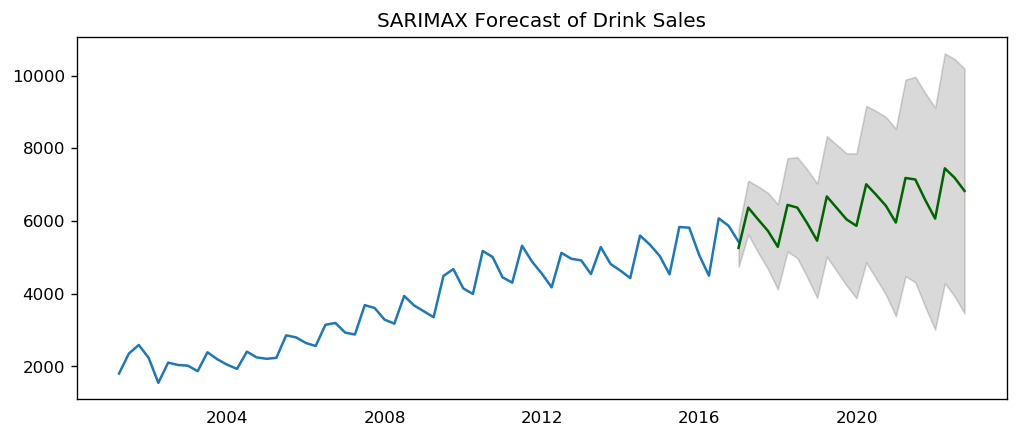
The coefficient of x1 is small and p-value is large, so the contribution from seasonal index is negligible.
Case Study
[64]:
df_drug = pd.read_csv(dataurl+'drug_sales.csv', parse_dates=['date'], index_col='date')
df_drug['year'] = [d.year for d in df_drug.index]
df_drug['month'] = [d.strftime('%b') for d in df_drug.index]
Python code cheat sheet:
Analysis:
df_drug.head()

plot_time_series(df_drug, 'sales', title='Drug Sales')

seasonal_plot(df_drug, ['month','sales'], title='Drug Sales')

boxplot(df_drug, ['month','sales'], title='Drug Sales')

stationarity_test(df_drug.sales, title='Drug Sales')

decomp(df_drug.sales)

detrend(df_drug['sales'])

deseasonalize(df_drug.sales, model, title='Drug Sales')
    #set model = 'multiplicative' or 'additive'#

plot_acf_pacf(df_drug.sales, acf_lag=50, pacf_lag=30)

differencing(df_drug, 'sales', title='Drug Sales')
SARIMA fitting and forecast:
sarima_drug = pm.auto_arima(df_drug.sales, start_p=1, start_q=1,
                         test='adf',
                         max_p=3, max_q=3, m=12,
                         start_P=0, seasonal=True,
                         d=None, D=1, trace=True,
                         error_action='ignore',
                         suppress_warnings=True,
                         stepwise=True)

sarima_drug.summary()

sarima_forcast(sarima_drug, df_drug, 'sales', forecast_periods=24, freq='month')
SARIMAX fitting and forecast:
df_drug = add_seasonal_index(df_drug, 'sales', freq='month', model='multiplicative')
sarimax_drug = pm.auto_arima(df_drug[['sales']], exogenous=df_drug[['seasonal_index']],
                           start_p=1, start_q=1,
                           test='adf',
                           max_p=3, max_q=3, m=12,
                           start_P=0, seasonal=True,
                           d=None, D=1, trace=True,
                           error_action='ignore',
                           suppress_warnings=True,
                           stepwise=True)

sarimax_drug.summary()

sarimax_forcast(sarimax_drug, df_drug, 'sales', forecast_periods=24, freq='month')