[1]:
%run initscript.py
%run ./files/loadoptfuncs.py
HTML("""
<div id="popup" style="padding-bottom:5px; display:none;">
<div>Enter Password:</div>
<input id="password" type="password"/>
<button onclick="done()" style="border-radius: 12px;">Submit</button>
</div>
<button onclick="unlock()" style="border-radius: 12px;">Unclock</button>
<a href="#" onclick="code_toggle(this); return false;">show code</a>
""")
[1]:
Optimization
All optimization models have several common elements:
Decision variables the variable whose values the decision maker is allowed to choose. The values of these variables determine such outputs as total cost, revenue, and profit.
An objective function (objective, for short) to be optimized – minimized or maximized.
Constraints that must be satisfied. They are usually physical, logical, or economic restrictions, depending on the nature of the problem.
In searching for the values of the decision variables that optimize the objective, only those values that satisfy all of the constraints are allowed.
To optimize means that you must systematically choose the values of the decision variables that make the objective as large (for maximization) or small (for minimization) as possible and cause all of the constraints to be satisfied.
Any set of values of the decision variables that satisfies all of the constraints is called a feasible solution. The set of all feasible solutions is called the feasible region.
Linear Programming
As one of the fundamental prescriptive analysis method, linear programming (LP) is used in all types of organizations, often on a daily basis, to solve a wide variety of problems such as advertising, distribution, investment, production, refinery operations, and transportation analysis.
More formally, linear programming is a technique for the optimization of a linear objective function, subject to linear equality and/or linear inequality constraints.
The main important feature of LP model is the presence of linearity in the problem. Some model may not be strictly linear, but can be made linear by applying appropriate mathematical transformations. Still some applications are not at all linear, but can be effectively approximated by linear models. LP models can be effectively solved by algorithms such as simplex, dual simplex and interior method. The ease with which LP models can usually be solved makes an attractive means of dealing with otherwise intractable nonlinear models.
Problem Formulation
The LP problem formulation is illustrated through a product mix problem.
A PC manufacturer assembles and then tests two models of computers, Basic and XP. There are at most 10,000 assembly hours at the cost of $11 available and 3000 testing hours at the cost of $15 available.
For each model, it has required assembly, testing hours, cost, price and estimated maximal sales.
Business assumptions:
No computers are in inventory from the previous period (or no beginning inventory)
Because these models are going to be changed after this month, the company doesn’t want to hold any inventory after this period (no ending inventory)
Business goal: the PC manufacturer wants to know
how many of each model it should produce
maximize its net profit
Business constraints:
resource constraints: available assembly and testing hours
market constraints: maximal sales
Algebraic Model
The PC manufacturer wants to
\begin{align*} \text{maximize} \quad \text{Profit} &= \text{Basic's unit margin} \times \text{Production of Basic} \\ & \qquad \qquad+ \text{XP's unit margin} \times \text{Production of XP} \end{align*}
subject to following constraints: \begin{align*} &\text{assembly hours:} & 5 \times \text{Production of Basic} + 6 \times \text{Production of XP} &\le 10000 \\ &\text{testing hours:} & \text{Production of Basic} + 2\times \text{Production of XP} &\le 3000 \\ &\text{maximal sales:} & \text{Production of Basic} &\le 600 \\ &\text{maximal sales:} & \text{Production of XP} &\le 1200 \\ \end{align*}
Intuitive constraints: \begin{align*} \text{Production of Basic} &\ge 0 \\ \text{Production of XP} &\ge 0 \\ \end{align*}
Graphical solution
When there are only two decision variables in an LP model, as there are in this product mix problem, we can demonstrate the problem graphically.
[2]:
interact(prodmix_graph,
zoom=widgets.Checkbox(value=False, description='Zoom In'));
We can modify objective coefficients in order to see how objective value changes in the feasible region.
[3]:
interact(prodmix_obj,
zoom=widgets.Checkbox(value=False, description='Zoom In', disabled=False),
margin1=widgets.IntSlider(min=-30,max=150,step=10,value=80,description='Margin Basic:',
style = {'description_width': 'initial'}),
margin2=widgets.IntSlider(min=-30,max=150,step=10,value=129,description='Margin XP:',
style = {'description_width': 'initial'}));
Because of this geometry, the optimal solution is always a corner point of the polygon. The simplex method for LP works so well because it can search through the finite number of corner points extremely efficiently and recognize when it has found the best corner point. This simple insight, plus its effective implementation in software package, has saved companies many millions of dollars.
Sensitivity Analysis
In any LP application, solving a model is simply the beginning of the analysis. It is always crucial to perform a sensitivity analysis to see how (or if) the optimal solution changes as one or more inputs vary. The sensitivity report from excel shows
Variable Cells
Name |
Reduced Cost |
Allowable Increase |
Allowable Decrease |
|---|---|---|---|
Number to produce Basic |
0 |
27.5 |
80 |
Number to produce XP |
33 |
1E+30 |
33 |
Final Value: the optimal solution.
Reduced Cost: it is relevant only if the final value is equal to either 0 or its upper bound. It indicates how much the objective coefficient of a decision variable (which is currently 0 or at its upper bound) must change before that variable changes.
For example: the number of XPs will stay at 1200 unless the profit margin for XPs decreases by at least $33.
Allowable Increase/Decrease: it indicates how much the objective coefficient could change before the optimal solution would change.
For example: if the selling price of Basics stays within a range from $220 to $327.5, the optimal product mix does not change at all.
Constraints
Name |
Shadow Price |
Allowable Increase |
Allowable Decrease |
|---|---|---|---|
Labor availability for assembling |
16 |
200 |
2800 |
Labor availability for testing |
0 |
1E+30 |
40 |
Final Value: the value of the left side of the constraint at the optimal solution.
Shadow Price: it indicates the change in the optimal value of the objective when the right side of some constraint changes by one unit.
For example: If the right side of this constraint increases by one hour, from 10000 to 10001, the optimal value of the objective will increase by $16.
SAS proc optmodel
In practice, users do not need to interact with solver directly. SAS, as well as many other software package, offers modeling language that allows the user to formulate the problem in algebraic model.
To try SAS optimization package, we can log into SAS on Demand cloud service through following procedures
Go to the link and click “Not registered or cannot sign in?”
Click “Don’t have a SAS Profile?”
Register a SAS account and login
Select enrollment tab and click “+ enroll in a course”
The course code is available by clicking “show answer”
[4]:
hide_answer()
[4]:
The course code is: d66f5458-24ac-44b3-8733-13f3ec9f3822
\(\blacksquare\)
Comparing to spreadsheet modeling, modeling language has a huge advantage because it can separate modeling and solution reporting from data management.
Datasets for a simple product mix problem
data ds_assemble;
input type $ cost avail;
datalines;
assemble 11 10000
;
run;
data ds_test;
input type $ cost avail;
datalines;
test 15 3000
;
run;
data ds_model;
input model $ assemble test cost price max_sale;
datalines;
Basic 5 1 150 300 600
XP 6 2 225 450 1200
;
run;
Datasets for a larger product mix problem
data ds_assemble;
input type $ cost avail;
datalines;
assemble 11 20000
;
run;
data ds_test;
input type $ cost avail;
datalines;
test1 19 5000
test2 17 6000
;
run;
data ds_model;
input model $ assemble test1 test2 cost price max_sale;
datalines;
Model1 4 1.5 2 150 350 1500
Model2 5 2 2.5 225 450 1250
Model3 5 2 2.5 225 460 1250
Model4 5 2 2.5 225 470 1250
Model5 5.5 2.5 3 250 500 1000
Model6 5.5 2.5 3 250 525 1000
Model7 5.5 2.5 3.5 250 530 1000
Model8 6 3 3.5 300 600 800
;
run;
The modeling code is quite general and can solve any product mix problem with given data structure.
proc optmodel;
/*read in data to set and arrays */
set<str> ASSEMBLE_LINES;
num assemble_cost{ASSEMBLE_LINES}, assemble_avail{ASSEMBLE_LINES};
read data ds_assemble into ASSEMBLE_LINES=[type] assemble_cost=cost assemble_avail=avail;
set<str> TEST_LINES;
num test_cost{TEST_LINES}, test_avail{TEST_LINES};
read data ds_test into TEST_LINES=[type] test_cost=cost test_avail=avail;
set<str> LABORS = ASSEMBLE_LINES union TEST_LINES;
set<str> MODELS;
num price{MODELS}, hours{MODELS,LABORS} , cost{MODELS}, max_sale{MODELS};
read data ds_model into MODELS=[model] {l in LABORS}<hours[model,l]=col(l)> cost price max_sale;
num margin{m in MODELS, t in TEST_LINES}
= price[m] - cost[m] - sum{a in ASSEMBLE_LINES} assemble_cost[a]*hours[m,a] - test_cost[t]*hours[m,t];
/* *********** * * * * * * *********** */
/* *********** build model *********** */
/* *********** * * * * * * *********** */
var Produce{m in MODELS, t in TEST_LINES} >=0;
/* production for each model in each testing line */
impvar Production_of_Model{m in MODELS} = sum{t in TEST_LINES} Produce[m,t];
/* implied variable: production for each model */
con Maximal_Sales{m in MODELS}:
Production_of_Model[m] <= max_sale[m];
/* total production for each model in all testing lines */
con Avail_Assemble{a in ASSEMBLE_LINES}:
sum{m in MODELS} hours[m,a]*Production_of_Model[m] <= assemble_avail[a];
con Avail_Test{t in TEST_LINES}:
sum{m in MODELS} hours[m,t]*Produce[m,t] <= test_avail[t];
max Profit=sum{m in MODELS, t in TEST_LINES} margin[m,t] * Produce[m,t];
solve;
create data solution from [t]=TEST_LINES {m in MODELS}<col(m)=Produce[m,t]>;
quit;
Mixed-Integer Programming
Optimization models in which some or all of the variables must be integer are known as mixed-integer programming (MIP). There are two main reasons for using MIP.
The decision variables are quantities that have to be integer, e.g., number of employee to assign or number of car to make
The decision variables are binaries to indicate whether an activity is undertaken, e.g., \(z=0\) or \(1\) where \(1\) indicates the decision of renting an equipment so that the firm need to pay a fixed cost, \(0\) otherwise.
If we relax the integrality requirements of MIP, then we obtain a so-called LP relaxation of a given MIP.
You might suspect that MIP would be easier to solve than LP models. After all, there are only a finite number of feasible integer solutions in an MIP model, whereas there are infinitely many feasible solutions in an LP model.
However, exactly the opposite is true. MIP models are considerably harder than LP models, because the optimal solution rarely occurs at the corner of its LP relaxation. Algorithms such as Branch-and-bound (B&B) or Branch-and-cut (B&C) are designed for solving MIP effectively and well implemented in commercial software.
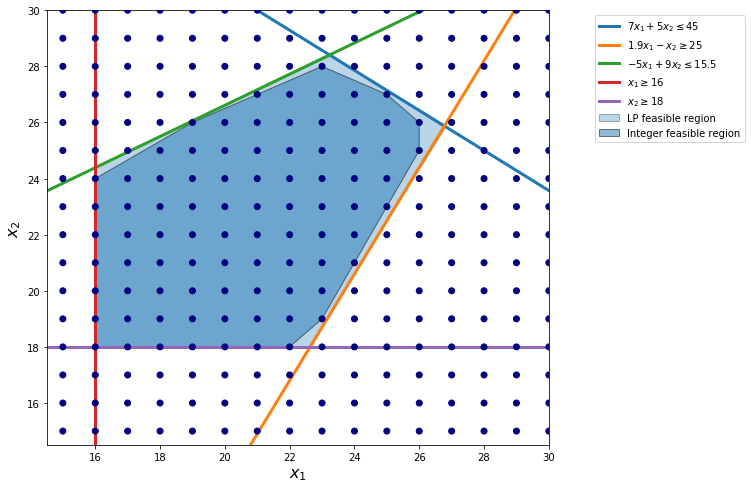
Branch and Bound Algorithm
Branch-and-bound algorithm is designed to use LP relaxation to solve MIP. The picture shows the difference between a MIP and its LP relaxation.
The “integer feasible region” in the picture connects all integer feasible solutions. In particular, it is a convex combination of all feasible solutions.
Similar to LP, the optimal solution of the MIP occurs at the corner of the integer feasible region.
However, as shown in the picture, the boundary of integer feasible region is much more complicated than its LP relaxation feasible region.
[5]:
show_integer_feasregion()
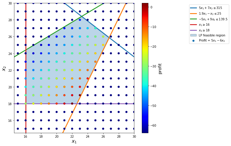
We demonstrate branch-and-bound procedure as follows.
[6]:
from ipywidgets import widgets
from IPython.display import display, Math
from traitlets import traitlets
class LoadedButton(widgets.Button):
"""A button that can holds a value as a attribute."""
def __init__(self, value=None, *args, **kwargs):
super(LoadedButton, self).__init__(*args, **kwargs)
# Create the value attribute.
self.add_traits(value=traitlets.Any(value))
def add_num(ex):
ex.value = ex.value+1
if ex.value<=3:
fig, ax = plt.subplots(figsize=(9, 8))
ax.set_xlim(15-0.5, 30)
ax.set_ylim(15-0.5, 30)
s = np.linspace(0, 50)
plt.plot(s, 45 - 5*s/7, lw=3, label='$5x_1 + 7x_2 \leq 315$')
plt.plot(s, -25 + 1.9*s, lw=3, label='$1.9x_1 - x_2 \leq 25$')
plt.plot(s, 15.5 + 5*s/9, lw=3, label='$-5x_1 + 9x_2 \leq 139.5$')
plt.plot(16 * np.ones_like(s), s, lw=3, label='$x_1 \geq 16$')
plt.plot(s, 18 * np.ones_like(s), lw=3, label='$x_2 \geq 18$')
# plot the possible (x1, x2) pairs
pairs = [(x1, x2) for x1 in np.arange(start=15, stop=31, step=1)
for x2 in np.arange(start=15, stop=31, step=1)]
# split these into our variables
x1, x2 = np.hsplit(np.array(pairs), 2)
# plot the results
plt.scatter(x1, x2, c=0*x1 - 0*x2, cmap='jet', zorder=3)
feaspairs = [(x1, x2) for x1 in np.arange(start=15, stop=31, step=1)
for x2 in np.arange(start=15, stop=31, step=1)
if (5/7*x1 + x2) <= 45
and (-1.9*x1 + x2) >= -25
and (-5/9*x1 + x2) <= 15.5
and x1>=16 and x2>=18]
# split these into our variables
x1, x2 = np.hsplit(np.array(feaspairs), 2)
# plot the results
plt.scatter(x1, x2, c=5*x1 - 6*x2, label='Profit = $5x_1 - 6x_2$', cmap='jet', zorder=3)
if ex.value>=3:
bpath1 = Path([
(16., 18.),
(16., 24.4),
(22, 27.8),
(22, 27),
(22, 18.),
(16., 18.),
])
bpatch1 = PathPatch(bpath1, label='New feasible region', alpha=0.5)
ax.add_patch(bpatch1)
bpath2 = Path([
(23., 18.7),
(23., 28.2),
(23.2,28.4),
(26.8, 25.8),
(23., 18.7),
])
bpatch2 = PathPatch(bpath2, label='New feasible region', alpha=0.5)
ax.add_patch(bpatch2)
cb = plt.colorbar()
cb.set_label('profit', fontsize=14)
plt.xlim(15-0.5, 30)
plt.ylim(15-0.5, 30)
plt.xlabel('$x_1$', fontsize=16)
plt.ylabel('$x_2$', fontsize=16)
lppath = Path([
(16., 18.),
(16., 24.4),
(23.3, 28.4),
(26.8, 25.8),
(22.6, 18.),
(16., 18.),
])
lppatch = PathPatch(lppath, label='LP feasible region', alpha=0.3)
ax.add_patch(lppatch)
if ex.value==1:
display(Math('Show~feasible~region...'))
if ex.value==2:
display(Math('Solve~linear~programming...'))
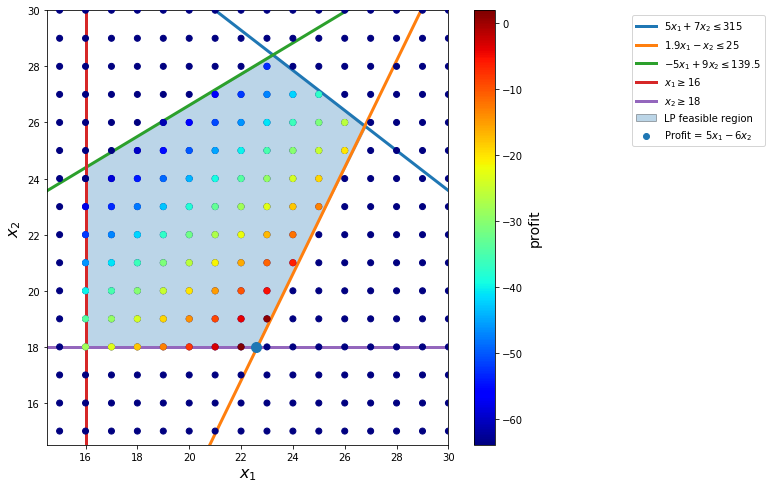
display(Math('\nThe~solution~is~x_1 = {:.3f}, x_2={}~with~profit={}'.format(22.632,18,5.158)))
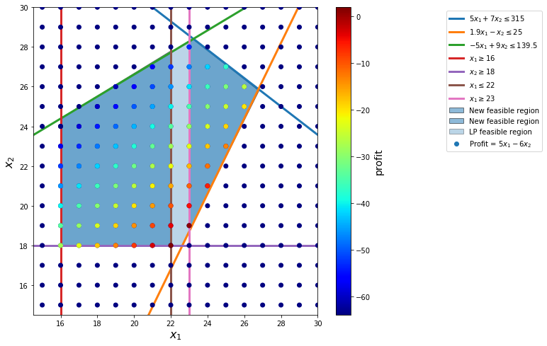
if ex.value==3:
display(Math('The~solution~is~integer~infeasible.~So~we~use~branch~and~bound.'))
display(Math('Branch~LP~feasible~region~into~two:~x_1 \le 22~and~x_1 \ge 23,~and~solve~two~LPs.'))
display(Math('Bound~the~optimal~profit~from~above~with~5.158.'))
if ex.value==2:
plt.scatter([22.57], [18], s=[100], zorder=4)
if ex.value>=3:
plt.plot(22 * np.ones_like(s), s, lw=3, label='$x_1 \leq 22$')
plt.plot(23 * np.ones_like(s), s, lw=3, label='$x_1 \geq 23$')
plt.legend(fontsize=18)
ax.legend(loc='upper right', bbox_to_anchor=(1.8, 1))
plt.show()
# lb = LoadedButton(description="Next", value=0)
# lb.on_click(add_num)
# display(lb)
class ex:
value = 1
for i in range(3):
ex.value = i
add_num(ex)
toggle()
[6]:
The Branch-and-bound algorithm keeps a tree structure in its solving process.
Modeling with Binary Variables
A binary variable usually corresponds to an activity that is or is not undertaken. We can model logics by using constraints involving binary variables.
For example, let \(z_1, \ldots, z_5\) be variables to indicate whether we will order products from suppliers \(1, \ldots, 5\) respectively.
The logic “if you use supplier 2, you must also use supplier 1” can be modeled as
\begin{align} z_2 \le z_1 \nonumber \end{align}
The logic “if you use supplier 4, you may NOT use supplier 5” can be modeled as
\begin{align} z_4 + z_5 \le 1 \nonumber \end{align}
Example
Consider the classic facility location problem. Given
a set \(L\) of customer locations and
a set \(F\) of candidate facility sites
We must decide on which sites to build facilities and assign coverage of customer demand to these sites so as to minimize cost.
All customer demand \(d_ i\) must be satisfied, and each facility has a demand capacity limit \(C\).
The total cost is the sum of the distances \(c_{ij}\) between facility \(j\) and its assigned customer \(i\), plus a fixed charge \(f_ j\) for building a facility at site \(j\).
Let \(y_ j = 1\) represent choosing site \(j\) to build a facility, and 0 otherwise. Also,
let \(x_{ij} = 1\) represent the assignment of customer \(i\) to facility \(j\), and 0 otherwise.
This model can be formulated as the following integer linear program:
Constraint (2) ensures that each customer is assigned to exactly one site.
Constraint (3) forces a facility to be built if any customer has been assigned to that facility.
Finally, constraint (4) enforces the capacity limit at each site.
\begin{align} \min & \quad \sum_{i \in L} \sum_{j \in F} c_{ij} x_{ij} + \sum_{j \in F} f_j y_j \\ \text{s.t.} & \quad \sum_{j \in F} x_{ij} = 1 && \forall i \in L \\ & \quad x_{ij} \leq y_j && \forall i \in L, j \in F \\ & \quad \sum_{i \in L} d_i x_{ij} \le C y_j && \forall j \in F \\ & \quad x_{ij} \in \{0,1\}, y_j \in \{0,1\} && \forall i \in L, j \in F \end{align}
SAS Log for MIP
NOTE: The Branch and Cut algorithm is using up to 2 threads.
Node Active Sols BestInteger BestBound Gap Time
0 1 5 13138.9827130 0 13139 0
0 1 5 13138.9827130 9946.2514269 32.10% 0
0 1 5 13138.9827130 9964.0867656 31.86% 0
0 1 5 13138.9827130 9972.4224200 31.75% 0
0 1 7 11165.8124056 9975.2866538 11.93% 0
0 1 7 11165.8124056 9977.8057106 11.91% 0
0 1 7 11165.8124056 9978.9372347 11.89% 0
0 1 7 11165.8124056 9980.8568737 11.87% 0
0 1 9 10974.7644641 9982.4953533 9.94% 0
NOTE: The MILP solver added 17 cuts with 492 cut coefficients at the root.
100 37 10 10961.8123535 10380.2158229 5.60% 0
121 44 11 10954.3760034 10938.0514190 0.15% 0
131 48 12 10951.0805543 10941.1165997 0.09% 0
139 49 13 10948.4603465 10941.1165997 0.07% 0
187 8 13 10948.4603465 10947.3813808 0.01% 0
NOTE: Optimal within relative gap.
NOTE: Objective = 10948.460347.
Although an MIP problem sometimes can be difficult to solve to its optimality, the gap column provides us useful information on solution quality. It shows that the objective value of the best integer solution the solver finds so far is within a certain percentage gap of the true underlying optimal solution.
Nonlinear Programming
In many optimization models the objective and/or the constraints are nonlinear functions of the decision variables. Such an optimization model is called a nonlinear programming (NLP) model.
When you solve an LP model, you are mostly guaranteed that the solution obtained is an optimal solution and a sensitivity analysis with shadow price and reduced cost is available.
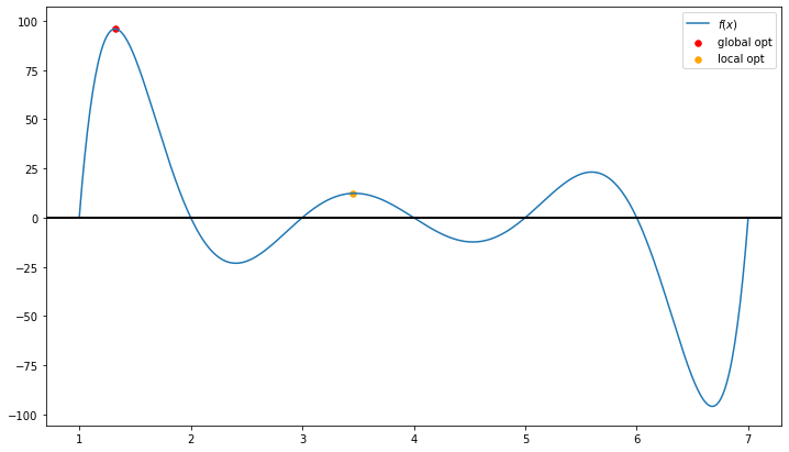
When you solve an NLP model, it is very possible that you obtain a suboptimal solution.
This is because a nonlinear function can have local optimal solutions where
a local optimum is better than all nearby points
that are not the global optimal solution
a global optimum is the best point in the entire feasible region
[7]:
draw_local_global_opt()
However, convex programming, as one of the most important type of nonlinear programming models, can be solved to its optimality.
[8]:
interact(showconvex,
values = widgets.FloatRangeSlider(value=[2, 3.5],
min=1.0, max=4.0, step=0.1,
description='Test:', disabled=False,
continuous_update=False,
orientation='horizontal',readout=True,
readout_format='.1f'));
Gradient Decent Algorithm
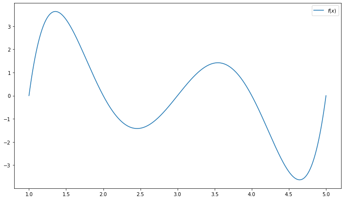
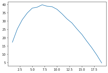
The gradient decent algorithm performs as the core part of many general purpose algorithms for solving NLP models. Consider a function
\begin{equation*} f(x) = (x-1) \times (x-2) \times (x-3) \times (x-4) \times (x-5) \end{equation*}
[9]:
function = lambda x: (x-1)*(x-2)*(x-3)*(x-4)*(x-5)
x = np.linspace(1,5,500)
plt.figure(figsize=(12,7))
plt.plot(x, function(x), label='$f(x)$')
plt.legend()
plt.show()
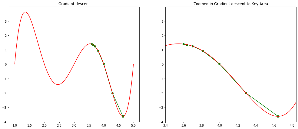
The gradient decent algorithm is typically used to find a local minimum with given initial solution. In our visual demonstration, a global optimal is found by using 3.6 as initial solution.
As it is usually impossible to identify the best initial solution, multistart option is often used in NLP solver, which will randomly select a large amount of initial solutions and run solver parallely.
[10]:
step(1.4, 0, 0.001, 0.05)
step(3.6, 0, 0.001, 0.05)
Local minimum occurs at: 2.4558826297046497
Number of steps: 11
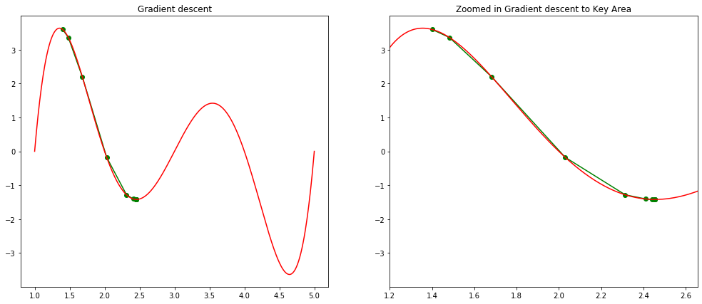
Local minimum occurs at: 4.644924463813627
Number of steps: 67
Genetic Algorithms
In the early 1970s, John Holland of the University of Michigan realized that many features espoused in the theory of natural evolution, such as survival of the fittest and mutation, could be used to help solve difficult optimization problems. Because his methods were based on behavior observed in nature, Holland coined the term genetic algorithm to describe his algorithm. Simply stated, a genetic algorithm (GA) provides a method of intelligently searching an optimization model’s feasible region for an optimal solution.
The process of natural selection starts with the selection of fittest individuals from a population. They produce offspring which inherit the characteristics of the parents and will be added to the next generation. If parents have better fitness, their offspring will be better than parents and have a better chance at surviving. This process keeps on iterating and at the end, a generation with the fittest individuals will be found.
[11]:
population = {
'A1': '000000',
'A2': '111111',
'A3': '101011',
'A4': '110110'
}
population
[11]:
{'A1': '000000', 'A2': '111111', 'A3': '101011', 'A4': '110110'}
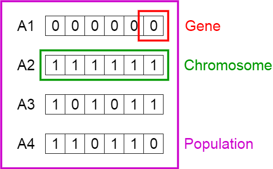
Biological terminology is used to describe the algorithm:
The objective function is called a fitness function.
An individual is characterized by a set of parameters known as Genes. Genes are joined into a string to form a Chromosome (variable or solution).
The set of genes of an individual is represented by using a string of binary values (i.e., string of \(1\)s and \(0\)s). We say that we encode the genes in a chromosome. For example,
1001 in binary system represents \(1 \times (2^3) + 0 \times (2^2) + 0 \times (2^1) + 1 \times (2^0) = 8 + 1 = 9\) in decimal system
It is similar to how 1001 is represented in decimal system \(1 \times (10^3) + 0\times (10^2) + 0 \times (10^1) + 1 \times (10^0) = 1000 + 1 = 1001\)
[12]:
{key:int(value,2) for key,value in population.items()}
[12]:
{'A1': 0, 'A2': 63, 'A3': 43, 'A4': 54}
GA uses the following steps: 1. Generate a population. The GA randomly samples values of the changing cells between the lower and upper bounds to generate a set of (usually at least 50) chromosomes. The initial set of chromosomes is called the population.
Create a new generation. Create a new generation of chromosomes in the hope of finding an improvement. In the new generation, chromosomes with a larger fitness function (in a maximization problem) have a greater chance of surviving to the next generation.
Crossover and mutation are also used to generate chromosomes for the next generation.
Crossover (fairly common) splices together two chromosomes at a pre-specified point.
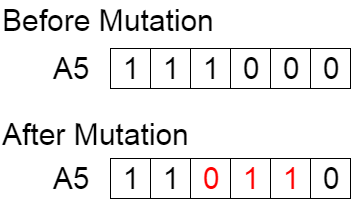
Mutation (very rare) randomly selects a digit and changes it from 0 to 1 or vice versa.
For example, consider the crossover point to be 3 as shown below.
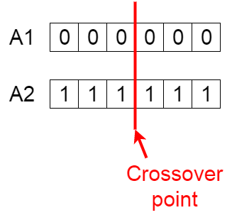
Offspring are created by exchanging the genes of parents among themselves until the crossover point is reached.
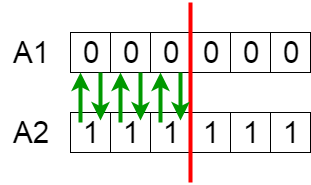
The new offspring A5 and A6 are added to the population.
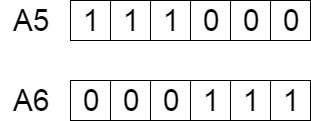
A5 may mutate
Stopping condition. At each generation, the best value of the fitness function in the generation is recorded, and the algorithm repeats step 2. If no improvement in the best fitness value is observed after many consecutive generations, the GA terminates.
Strengths of GA:
If you let a GA run long enough, it is guaranteed to find the solution to any optimization problem.
GAs do very well in problems with few constraints. The complexity of the objective cell does not bother a GA. For example, a GA can easily handle MIN, MAX, IF, and ABS functions in the models. This is the key advantage of GAs.
Weakness of GA:
It might take too long to find a good solution. Even a solution is found, you do not know if the solution is optimal or how close it is to the optimal solution.
GAs do not usually perform very well on problems that have many constraints. For example, Simplex LP Solver has no difficulty with the multiple-constraint linear models, but GAs perform much worse and more slowly on them.
Operations Research
Operations research is a discipline that deals with the application of advanced analytical methods to help make better decisions. It is often considered to be a sub-field of applied mathematics. The terms management science and decision science are sometimes used as synonyms.
Employing techniques of predictive and prescriptive analysis, such as mathematical modeling, statistical analysis, and mathematical optimization, operations research arrives at optimal or near-optimal solutions to complex decision-making problems.
Because of its emphasis on human-technology interaction and because of its focus on practical applications, operations research has overlap with other disciplines, notably industrial engineering and operations management, and draws on psychology and organization science.
Operations research is often concerned with determining the extreme values of some real-world objective: the maximum (of profit, performance, or yield) or minimum (of loss, risk, or cost). Originating in military efforts during World War II, its techniques have grown to concern problems in a variety of industries.
Operations research often models a decision process as an optimization problem
\begin{align*} \min & \quad f(x) \\ \text{subject to} & \quad h_i(x) \geq 0 \quad \forall i = 1, \ldots, n \end{align*}
If the objective function and constraints are all convex functions, then it is a convex problem, otherwise it is a non-convex problem.
In general, commercial software, such as CPLEX or Gurobi,
can find an optimal solution for convex problem, for example, linear programming.
use branch-and-bound algorithm to solve mixed-integer programming, which is generally a non-convex problem. Although it cannot guarantee a global optimal solution, it can provide an optimality gap to show the solution quality.
can only find a local optimal for general non-convex problem without knowing solution quality.
Traveling Salesman Problem (TSP)
The TSP has several applications even in its purest formulation, such as planning, logistics, and the manufacture of microchips. TSP is a touchstone for many general heuristics devised for combinatorial optimization such as genetic algorithms.
For example, UPS has invested heavily in a project, called On-Road Integrated Optimization and Navigation (ORION) based on TSP, that it says will shorten drivers’ routes and save millions on fuel.
Blending Problem
Blending models can be used to find the optimal combination of outputs as well as the mix of inputs that are used to produce the desired outputs.
The model is adopted into a tool called Petro in Chevron. Petro has strongly influenced the way their downstream business approaches planning and decision making; it is an integral part of Chevron’s processes and culture.
Scheduling
Scheduling is the process of arranging, controlling and optimizing work and workloads in a production process or manufacturing process. Optimization is well implemented in all types of scheduling problems, such as sports scheduling.
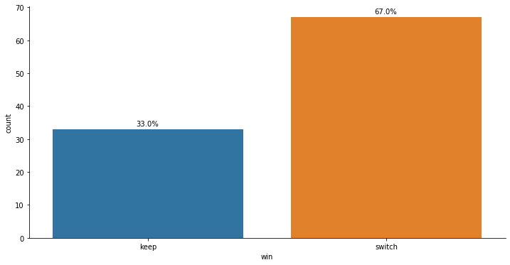
Monty Hall Problem
The problem is well described in movie 21. The simulation game can be played in this link.
Without loss of generality, we assume that the player always selects door 1 at the beginning of the game. The simulation shows that the “switch” strategy achieves a higher probability for winning the car.
[13]:
widgets.interact_manual.opts['manual_name'] = 'Run Simulation'
interact_manual(montyhall,
sample_size=widgets.BoundedIntText(value=100, min=100, max=10000,
description='Sample Size:', disabled=False));
montyhall(100)
| door1 | door2 | door3 | select | keep | prize | open | switch | win | |
|---|---|---|---|---|---|---|---|---|---|
| 0 | goat | goat | car | 1 | 1 | 3 | 2 | 3 | switch |
| 1 | goat | car | goat | 1 | 1 | 2 | 3 | 2 | switch |
| 2 | car | goat | goat | 1 | 1 | 1 | 3 | 2 | keep |
| 3 | goat | car | goat | 1 | 1 | 2 | 3 | 2 | switch |
| 4 | car | goat | goat | 1 | 1 | 1 | 3 | 2 | keep |
| 5 | goat | goat | car | 1 | 1 | 3 | 2 | 3 | switch |
| 6 | goat | goat | car | 1 | 1 | 3 | 2 | 3 | switch |
| 7 | goat | car | goat | 1 | 1 | 2 | 3 | 2 | switch |
| 8 | goat | goat | car | 1 | 1 | 3 | 2 | 3 | switch |
| 9 | goat | car | goat | 1 | 1 | 2 | 3 | 2 | switch |
Secretary Problem
Imagine you’re interviewing a set of applicants for a position as a secretary, and your goal is to maximize the chance of hiring the single best applicant in the pool. While you have no idea how to assign scores to individual applicants, you can easily judge which one you prefer. You interview the applicants one at a time. You can decide to offer the job to an applicant at any point and they are guaranteed to accept, terminating the search. But if you pass over an applicant, deciding not to hire them, they are gone forever. The simulation game can be played in this link.
In your search for a secretary, there are two ways you can fail: stopping early and stopping late. When you stop too early, you leave the best applicant undiscovered. When you stop too late, you hold out for a better applicant who doesn’t exist.
The optimal solution takes the form of the Look-Then-Leap Rule:
You set a predetermined amount of time for “looking”, that is, exploring your options, gathering data — in which you categorically don’t choose anyone, no matter how impressive.
After that point, you enter the “leap” phase, prepared to instantly commit to anyone who outshines the best applicant you saw in the look phase.
We can see how the Look-Then-Leap Rule emerges by considering how the secretary problem plays out in a small applicant pool.
[14]:
hide_answer()
[14]:
One applicant the problem is easy to solve — hire her!
With two applicants, you have a 50% chance of success no matter what you do. You can hire the first applicant (who’ll turn out to be the best half the time), or dismiss the first and by default hire the second (who is also best half the time).
Add a third applicant, and all of a sudden things get interesting. Can we do better than chance which is 33%?
When we see the first applicant, we have no information — she’ll always appear to be the best yet.
When we see the third applicant, we have no agency — we have to make an offer to the final applicant.
For the second applicant, we have a little bit of both: we know whether she is better or worse than the first, and we have the freedom to either hire or dismiss her.
What happens when we just hire her if she’s better than the first applicant, and dismiss her if she’s not? This turns out to be the best possible strategy with 50% of chance getting the best candidate.
Suppose there are three candidates: Best, Good, Bad. There are 6 possible orders:
Best, Good, Bad: hire Bad (the last one)
Best, Bad, Good: hire Good (the last one)
Good, Best, Bad: hire Best
Good, Bad, Best: hire Best
Bad, Best, Good: hire Best
Bad, Good, Best: hire Good
\(\blacksquare\)
[15]:
successful_rate(5, [2], printtable=True)
The best candidate is hired 2171 times in 5000 trials with 2 rejection
| person1 | person2 | person3 | person4 | person5 | best_score | best | best_at_stop | hired_score | hired | |
|---|---|---|---|---|---|---|---|---|---|---|
| 0 | 40 | 35 | 81 | 61 | 98 | 98 | person5 | 40 | 81 | person3 |
| 1 | 14 | 51 | 45 | 13 | 52 | 52 | person5 | 51 | 52 | person5 |
| 2 | 75 | 65 | 72 | 19 | 44 | 75 | person1 | 75 | 44 | person5 |
| 3 | 96 | 20 | 29 | 83 | 86 | 96 | person1 | 96 | 86 | person5 |
| 4 | 61 | 79 | 59 | 52 | 18 | 79 | person2 | 79 | 18 | person5 |
| 5 | 73 | 63 | 85 | 83 | 4 | 85 | person3 | 73 | 85 | person3 |
| 6 | 86 | 70 | 61 | 94 | 15 | 94 | person4 | 86 | 94 | person4 |
| 7 | 97 | 23 | 86 | 76 | 44 | 97 | person1 | 97 | 44 | person5 |
| 8 | 14 | 86 | 61 | 65 | 40 | 86 | person2 | 86 | 40 | person5 |
| 9 | 20 | 2 | 66 | 28 | 10 | 66 | person3 | 20 | 66 | person3 |
[15]:
{2: 43.419999999999995}
[16]:
style = {'description_width': '150px'}
widgets.interact_manual.opts['manual_name'] = 'Run Simulation'
interact_manual(secretary,
n=widgets.BoundedIntText(value=20, min=5, max=100,
description='number of candidates:', disabled=False, style=style));
secretary(20);
optimal rejection is 7 with 40.0% chance to hire the best candidate
The optimal rule is the 37% Rule: look at the first 37% of the applicants, choosing none, then be ready to leap for anyone better than all those you’ve seen so far. To be precise, the mathematically optimal proportion of applicants to look at is \(1/e\). So, anything between 35% and 40% provides a success rate extremely close to the maximum.
In the secretary problem we know nothing about the applicants other than how they compare to one another. Some variations of the problem are studied:
If every secretary, for instance, had a GRE scored, which is the only thing that matters about our applicants. Then, we should use the Threshold Rule, where we immediately accept an applicant if she is above a certain percentile.
If waiting has a cost measured in dollars, a good candidate today beats a slightly better one several months from now.
If we have ability to recall a past candidate.