[1]:
%run initscript.py
%run ./files/loadmlfuncs.py
HTML("""
<div id="popup" style="padding-bottom:5px; display:none;">
    <div>Enter Password:</div>
    <input id="password" type="password"/>
    <button onclick="done()" style="border-radius: 12px;">Submit</button>
</div>
<button onclick="unlock()" style="border-radius: 12px;">Unclock</button>
<a href="#" onclick="code_toggle(this); return false;">show code</a>
""")
[1]:
Machine Learning
Logistic Regression
Logistic regression is a popular method for classifying individuals (although we call it regression), given the values of a set of explanatory variables. It estimates the probability that an individual is in a particular category. We will demonstrate the method by considering a book club case.
In a book club, a new title, “The Art History of Florence”, is ready for release. The book club has sent promotion mails to a sample of customers from its customer base in two different times. Each time it randomly select 1000 customers.
[2]:
df_book_part1 = pd.read_csv(dataurl+'book_train.csv', header=0, index_col='customer')
df_book_part2 = pd.read_csv(dataurl+'book_validation.csv', header=0, index_col='customer')
display(df_book_part1.head())
display(df_book_part2.tail())
| month | art_book | purchased | |
|---|---|---|---|
| customer | |||
| 1 | 24 | 0 | 0 |
| 2 | 16 | 0 | 0 |
| 3 | 15 | 0 | 0 |
| 4 | 22 | 0 | 0 |
| 5 | 15 | 0 | 1 |
| month | art_book | purchased | |
|---|---|---|---|
| customer | |||
| 1996 | 9 | 1 | 1 |
| 1997 | 9 | 0 | 0 |
| 1998 | 28 | 1 | 0 |
| 1999 | 6 | 1 | 0 |
| 2000 | 10 | 0 | 0 |
The book club has collected several variables for all 2000 customers as follows:
month: months to the customer’s last purchase when promotion mail is sent
art_book: number of art books the customer purchased before
purchased: if s/he paid for the new title “The Art History of Florence”
It costs the book club $1 for sending a mail and generates $7 profit for selling the book. After two promotions, the manager of the book club realizes that the store actually lose money in both promotions.
[3]:
def calc_profit(df):
    mail_cost = 1
    selling_profit = 7
    profit = df.purchased.sum() * 7 - df.month.count()*mail_cost
    return profit

print('net profit for the 1st promotion:', calc_profit(df_book_part1))
print('net profit for the 2nd promotion:', calc_profit(df_book_part2))
net profit for the 1st promotion: -419
net profit for the 2nd promotion: -433
The manager was wondering if the book club could use a predictive model to predict each customer’s probability of purchasing. Then, the store may only send out promotion mails to customers with a high chance of purchasing. In order to prove the concept, the manager starts with two questions:
can we derive a prediction model after collecting the data from the first promotion?
can this prediction model improve the second promotion?
We expect that this prediction model can
utilize
monthandart_bookto predictpurchased
which suggests a regression equation purchased \(\sim\) month \(+\) art_book. However, the \(y\) variable purchased is either 0 or 1, and a scatter plot between purchased and month (\(y\) vs \(x\)) shows as follows
[4]:
df_book_part1.plot.scatter(x='month', y='purchased')
plt.show()
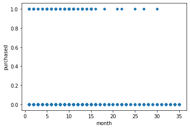
The graph is against many linear regression assumptions such as
there is no linear relationship between independent and dependent variables.
error term is probably not normally distributed.
Instead of using the binary variable (purchased or not), we may consider purchasing probability \(p\) as dependent variable in a regression equation such as
\begin{align} p &= \beta_0 + \beta_1 \times \text{month} + \beta_2 \times \text{art_book} \end{align}
Although \(p\) is continuous, we still cannot run a linear regression on \(p\) because it is bounded in range \([0,1]\). In linear regression, the dependent variable should be able to take any value in range \([-\infty, +\infty]\).
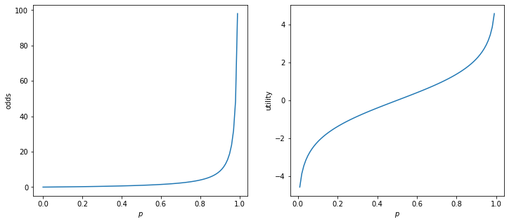
We introduce odds and utility
\begin{align} \text{odds} &= \frac{p}{1-p} \nonumber \\ \text{utility} &= \log(\text{odds}) \nonumber \\ \end{align}
Note that utility is in \([-\infty, +\infty]\). Now a regression equation can be used
\begin{align} \text{utility} &= \beta_0 + \beta_1 \times \text{month} + \beta_2 \times \text{art_book} \end{align}
[5]:
p = np.linspace(0,1,100)
odds = p / (1-p)
utility = np.log(odds)

plt.subplots(1, 2, figsize=(12,5))
plt.subplot(1, 2, 1)
plt.plot(p, odds)
plt.xlabel('$p$')
plt.ylabel('odds')

plt.subplot(1, 2, 2)
plt.plot(p, utility)
plt.xlabel('$p$')
plt.ylabel('utility')

plt.show()
toggle()
[5]:
In practice, we can simply use logistic regression to deal with binary dependent variable. Statistical tools will perform all the transformation for us after we provide the regression equation purchased \(\sim\) month \(+\) art_book. In python, we can use either statmodels which provides statistical summary or sklearn package.
[6]:
from statsmodels.api import add_constant
import statsmodels.api as sm
X = add_constant(df_book_part1[['month','art_book']])
y = df_book_part1['purchased']
model = sm.Logit(y, X)
model.fit().summary()
Optimization terminated successfully.
         Current function value: 0.251466
         Iterations 7
[6]:
| Dep. Variable: | purchased | No. Observations: | 1000 |
|---|---|---|---|
| Model: | Logit | Df Residuals: | 997 |
| Method: | MLE | Df Model: | 2 |
| Date: | Wed, 04 Sep 2019 | Pseudo R-squ.: | 0.1209 |
| Time: | 20:34:59 | Log-Likelihood: | -251.47 |
| converged: | True | LL-Null: | -286.04 |
| Covariance Type: | nonrobust | LLR p-value: | 9.698e-16 |
| coef | std err | z | P>|z| | [0.025 | 0.975] | |
|---|---|---|---|---|---|---|
| const | -2.2256 | 0.239 | -9.315 | 0.000 | -2.694 | -1.757 |
| month | -0.0707 | 0.019 | -3.677 | 0.000 | -0.108 | -0.033 |
| art_book | 0.9891 | 0.135 | 7.345 | 0.000 | 0.725 | 1.253 |
The signs of the coefficients indicate whether the probability of purchasing the book increases or decreases when these variables increases. For example, the probability of purchasing the book decrease as month increase (because of its minus sign) and increase as art_book increase (because of its plus sign).
However, you have to use caution when interpreting the magnitudes of the coefficients. For example, the absolute value of coefficient of month is smaller than art_book because month generally have larger values than art_book.
The value \(\exp\)(coefficient) is more interpretable. For example, if art_book increases 1, the odds of purchasing the book increase by a factor about \(\exp(0.9888)\). So, you should be on the lookout for values well above or below 1.
[7]:
from sklearn import linear_model

X = df_book_part1[['month','art_book']]
y = df_book_part1['purchased']

clf = linear_model.LogisticRegression(C=1e5, solver='lbfgs')
clf.fit(X, y)
print('intercept=', clf.intercept_, '\ncoefficient =', clf.coef_)
intercept= [-2.22563221]
coefficient = [[-0.07071734  0.98904918]]
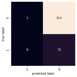
The classification matrix is
[8]:
from sklearn.metrics import confusion_matrix

labels = clf.predict(df_book_part1[['month','art_book']])
mat = confusion_matrix(df_book_part1['purchased'], labels)
sns.heatmap(np.flip(mat), square=True, annot=True, fmt='d', cbar=False,
            xticklabels=[1,0], yticklabels=[1,0])
plt.xlabel('predicted label')
plt.ylabel('true label')
plt.ylim(0,mat.shape[0])
plt.show()
toggle()
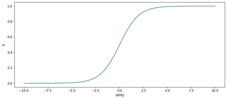
[8]:
After we have obtained \(\beta_0, \beta_1\) and \(\beta_2\), we can use equation \((2)\) for our validation data to evaluate its utility. Then, the probability can be derived by
\begin{align} p = \frac{\exp(\text{utility})}{1+\exp(\text{utility})} \nonumber \end{align}
[9]:
utility = np.linspace(-10,10,100)
p = np.exp(utility) / (1 + np.exp(utility))

plt.subplots(1, 1, figsize=(12,5))
plt.plot(utility, p)
plt.xlabel('utility')
plt.ylabel('$p$')
plt.show()
toggle()
[9]:
In general, our decision can be made based on a threshold value 0.5. That is, if the probability that a customer may purchase the book is greater than 0.5, we send a mail.
However, in the book club case, it has a simple break-even point where the cost-profit ratio is \(1/7\). Therefore, our strategy can be designed based on this ratio as follows. If the probability that a customer may purchase the book is greater than \(1/7\), we send a mail, otherwise we do not.
We prefer to use sklearn because it provides capability to predict the probability directly.
[10]:
df_book_part2['purchase_prob'] = clf.predict_proba(df_book_part2[['month','art_book']])[:,1]
df_book_part2['send'] = df_book_part2['purchase_prob'] > 1/7
df_book_part2.head()
[10]:
| month | art_book | purchased | purchase_prob | send | |
|---|---|---|---|---|---|
| customer | |||||
| 1001 | 30 | 0 | 0 | 0.012778 | False |
| 1002 | 12 | 0 | 0 | 0.044182 | False |
| 1003 | 18 | 0 | 0 | 0.029354 | False |
| 1004 | 27 | 1 | 0 | 0.041251 | False |
| 1005 | 4 | 1 | 0 | 0.179542 | True |
[11]:
num_mail_send = df_book_part2[df_book_part2['send']].shape[0]
num_purchased = df_book_part2[df_book_part2['send'] & df_book_part2['purchased'] == 1].shape[0]
profit = num_purchased * 7 - num_mail_send
print('Based on our prediction model, we should send {} mails.'.format(num_mail_send))
print('We would expect receiving {} orders and our profit is ${}.'.format(num_purchased, profit))
toggle()
Based on our prediction model, we should send 128 mails.
We would expect receiving 38 orders and our profit is $138.
[11]:
Naive Bayes
Naive Bayes models are a group of extremely fast and simple classification algorithms that are often suitable for very high-dimensional datasets. Because they are so fast and have so few tunable parameters, they end up being very useful as a quick-and-dirty baseline for a classification problem. This section will focus on an intuitive explanation of how naive Bayes classifiers work.
Naive Bayes classifiers are built on Bayesian classification methods. These rely on Bayes’s theorem, which is an equation describing the relationship of conditional probabilities of statistical quantities.
In Bayesian classification, we’re interested in finding the probability of a label given some observed features, which we can write as \(P(C~|~{\rm features})\). Bayes’s theorem tells us how to express this in terms of quantities we can compute more directly:
If we are trying to decide between two labels — let’s call them \(C_1\) and \(C_2\) — then one way to make this decision is to compute the ratio of the posterior probabilities for each label:
All we need now is some model by which we can compute \(P({\rm features}~|~C_i)\) for each label. Such a model is called a generative model because it specifies the hypothetical random process that generates the data.
Specifying this generative model for each label is the main piece of the training of such a Bayesian classifier. The general version of such a training step is a very difficult task, but we can make it simpler through the use of some simplifying assumptions about the form of this model.
This is where the “naive” in “naive Bayes” comes in: if we make very naive assumptions about the generative model for each label, we can find a rough approximation of the generative model for each class, and then proceed with the Bayesian classification.
Bernoulli Naive Bayes
We revisit the book club case with an updated dataset. Now the data includes two categorical dependent variables gender and married as additional explanatory variables. The dataset is partitioned into training and testing datasets.
[12]:
df_book = pd.read_csv(dataurl+'book_club.csv', header=0)
df_book_train = df_book.iloc[:1000]
df_book_test = df_book.iloc[1000:]
df_book.head(8)
toggle()
[12]:
For the Naive Bayes method, numeric predictors must be binned, i.e., made categorical. For this example, each numeric variable has been binned by its quartiles as shown below. It is important to note that the quartiles are calculated based on the training dataset.
[13]:
df_quantile = df_book_train[['month', 'art_book']].quantile([0, .25, .5, .75, 1]).astype('int64')
df_quantile['quantile'] = range(len(df_quantile))
df_book_train = transfer_data(df_book_train, df_quantile)
df_book_test = transfer_data(df_book_test, df_quantile)
display(df_quantile)
toggle()
| month | art_book | quantile | |
|---|---|---|---|
| 0.00 | 1 | 0 | 0 |
| 0.25 | 7 | 0 | 1 |
| 0.50 | 12 | 0 | 2 |
| 0.75 | 15 | 1 | 3 |
| 1.00 | 35 | 5 | 4 |
[13]:
Our goal is to classify customers into different classes (purchased is either 0 or 1) based on their features. We count frequency of each feature in each class based on the training data.
[14]:
def frequency_count(col, normalize):
    return df_book_train.groupby('purchased')[col].value_counts(normalize=normalize).sort_index()

interact(frequency_count,
         col=widgets.Dropdown(options=df_book_train.columns, value='gender', description='column:',disabled=False),
         normalize=widgets.Checkbox(value=False, description='normalize',disabled=False)
        );
toggle()
[14]:
The normalized frequency provides the probability of a feature given an individual’s class. For example, person 1 has purchased = 0 and gender = “FEMALE”. We obtain a probability
\begin{align} p(\text{gender $=$ 'FEMALE'}|\text{purchased}=0) = \frac{\text{# of females and purchased $=$ 0}}{\text{# of persons with purchased $=$ 0}} = 0.676 \nonumber \end{align}
The value (0, “FEMALE”): 0.676 shows that, if a customer did not purchase the new book, the probability of his/her gender being female is 0.676.
Similarly, we can calculate
\begin{align*} &p(\text{gender $=$ 'MALE'}|\text{purchased}=0) \\ &p(\text{gender $=$ 'FEMALE'}|\text{purchased}=1) \\ &p(\text{married $=$ 'YES'}|\text{purchased}=0) \\ &p(\text{married $=$ 'No'}|\text{purchased}=1) \\ &p(\text{month $=$ 3}|\text{purchased}=0) \\ &p(\text{art_book $=$ 2}|\text{purchased}=1) \end{align*}
and so on. In summary, we have \(p(\text{feature}|\text{purchased}=0)\) and \(p(\text{feature}|\text{purchased}=1)\) for each possible feature of all customers. All the probabilities can be considered as a feature dictionary.
With this feature dictionary, we want to obtain probabilities
\begin{align} p(\text{customer } i|\text{purchased}=0) \text{ and } p(\text{customer } i|\text{purchased}=1) \nonumber \end{align}
where the probability \(p(\text{customer } i|\text{purchased}=0)\) can be interpret as
if a customer did not purchase the new book, s/he has probability \(p(\text{customer } i|\text{purchased}=0)\) being customer 1.
Then our prediction is as simple as follows
If \(p(\text{customer } i|\text{purchased}=0) > p(\text{customer } i|\text{purchased}=1)\) then we prediction the customer will not purchase the new book,
Otherwise, we prediction the customer will purchase the new book.
Here is how probabilities \begin{align} p(\text{customer 1}|\text{purchased}=0) \text{ and } p(\text{customer 1}|\text{purchased}=1) \nonumber \end{align}
are calculated. For customer 1,
\begin{align*} p(\text{customer 1}|\text{purchased}=0) = & p(\text{month}=3|\text{purchased}=0) \\ & \times p(\text{art_book}=2|\text{purchased}=0) \\ & \times p(\text{gender $=$ FEMALE}|\text{purchased}=0) \\ & \times p(\text{married $=$ Yes}|\text{purchased}=0) \end{align*}
and
\begin{align*} p(\text{customer 1}|\text{purchased}=1) = & p(\text{month}=3|\text{purchased}=1) \\ & \times p(\text{art_book}=2|\text{purchased}=1) \\ & \times p(\text{gender $=$ FEMALE}|\text{purchased}=1) \\ & \times p(\text{married $=$ Yes}|\text{purchased}=1) \end{align*}
Note that we assume all the features are independent so that a simple multiplication can be applied (that is why this method is called naive). Thus, \(p(\text{customer 1}|\text{purchased}=0)\) is the probability to have the exactly same features as customer 1 if a random person did not purchase the new book.
[15]:
def predict(df):
    df['prediction'] = [0
        if np.prod([dict(frequency_count(col, True))[(0,df.iloc[row][col])]
                    if (0,df.iloc[row][col]) in dict(frequency_count(col, True)).keys()
                    else 0
                    for col in df.columns if col not in ['purchased','prediction']]) > \
           np.prod([dict(frequency_count(col, True))[(1,df.iloc[row][col])]
                    if (1,df.iloc[row][col]) in dict(frequency_count(col, True)).keys()
                    else 0
                    for col in df.columns if col not in ['purchased','prediction']])\
        else 1
                   for row in range(df.shape[0])]

predict(df_book_test)
display(df_book_test.head(8))
display(df_book_test.groupby(['prediction','purchased']).size().unstack(level=1, fill_value=0))
toggle()
| gender | married | purchased | month | art_book | prediction | |
|---|---|---|---|---|---|---|
| customer | ||||||
| 1001 | MALE | YES | 0 | 3 | 2 | 0 |
| 1002 | FEMALE | YES | 0 | 2 | 2 | 0 |
| 1003 | FEMALE | YES | 0 | 3 | 2 | 0 |
| 1004 | MALE | YES | 0 | 3 | 3 | 0 |
| 1005 | MALE | NO | 0 | 0 | 3 | 1 |
| 1006 | MALE | YES | 0 | 4 | 2 | 0 |
| 1007 | MALE | YES | 0 | 0 | 2 | 0 |
| 1008 | MALE | YES | 0 | 3 | 2 | 0 |
| purchased | 0 | 1 |
|---|---|---|
| prediction | ||
| 0 | 701 | 26 |
| 1 | 218 | 55 |
[15]:
The predictive model suggests sending 273 = (218 + 55) mails. We would expect receiving 55 orders and our profit is $112.
Multinomial Naive Bayes
In multinomial naive Bayes, the features are assumed to be generated from a simple multinomial distribution.
The multinomial distribution describes the probability of observing counts among a number of categories, and thus multinomial naive Bayes is most appropriate for features that represent counts or count rates.
The idea is precisely the same as before, except that instead of modeling the data distribution with the best-fit Gaussian, we model the data distribution with a best-fit multinomial distribution.
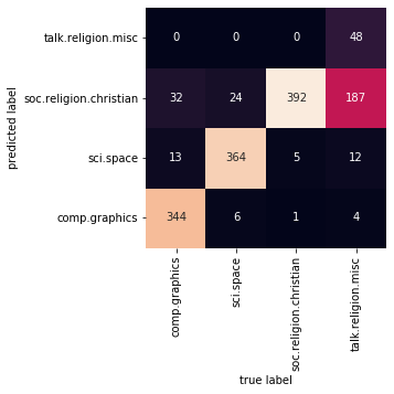
One place where multinomial naive Bayes is often used is in text classification, where the features are related to word counts or frequencies within the documents to be classified.
Here we will use the sparse word count features from the 20 Newsgroups corpus to show how we might classify these short documents into categories.
[16]:
from sklearn.datasets import fetch_20newsgroups

data = fetch_20newsgroups()
display(data.target_names)

# choose a subset categories to learn
categories = ['talk.religion.misc',
              'soc.religion.christian',
              'sci.space',
              'comp.graphics']

train = fetch_20newsgroups(subset='train', categories=categories)
test = fetch_20newsgroups(subset='test', categories=categories)
['alt.atheism',
 'comp.graphics',
 'comp.os.ms-windows.misc',
 'comp.sys.ibm.pc.hardware',
 'comp.sys.mac.hardware',
 'comp.windows.x',
 'misc.forsale',
 'rec.autos',
 'rec.motorcycles',
 'rec.sport.baseball',
 'rec.sport.hockey',
 'sci.crypt',
 'sci.electronics',
 'sci.med',
 'sci.space',
 'soc.religion.christian',
 'talk.politics.guns',
 'talk.politics.mideast',
 'talk.politics.misc',
 'talk.religion.misc']
Here is a representative entry from the data:
[17]:
print(train.data[5])
From: dmcgee@uluhe.soest.hawaii.edu (Don McGee)
Subject: Federal Hearing
Originator: dmcgee@uluhe
Organization: School of Ocean and Earth Science and Technology
Distribution: usa
Lines: 10


Fact or rumor....?  Madalyn Murray O'Hare an atheist who eliminated the
use of the bible reading and prayer in public schools 15 years ago is now
going to appear before the FCC with a petition to stop the reading of the
Gospel on the airways of America.  And she is also campaigning to remove
Christmas programs, songs, etc from the public schools.  If it is true
then mail to Federal Communications Commission 1919 H Street Washington DC
20054 expressing your opposition to her request.  Reference Petition number

2493.
[18]:
from sklearn.feature_extraction.text import TfidfVectorizer
from sklearn.naive_bayes import MultinomialNB
from sklearn.pipeline import make_pipeline
from sklearn.metrics import confusion_matrix

# Fit the model and show the classification matrix
#convert the content of each string into a vector of numbers
model = make_pipeline(TfidfVectorizer(), MultinomialNB())
model.fit(train.data, train.target)
labels = model.predict(test.data)
mat = confusion_matrix(test.target, labels)
sns.heatmap(mat.T, square=True, annot=True, fmt='d', cbar=False,
            xticklabels=train.target_names, yticklabels=train.target_names)
plt.xlabel('true label')
plt.ylabel('predicted label')
plt.ylim(0, mat.shape[0])
plt.show()

def predict_category(s, train=train, model=model):
    pred = model.predict([s])
    return train.target_names[pred[0]]
toggle()
[18]:
Evidently, even this very simple classifier can successfully separate space talk from computer talk, but it gets confused between talk about religion and talk about Christianity. This is perhaps an expected area of confusion!
The very cool thing here is that we now have the tools to determine the category for any string, using the predict() method of this pipeline. Here’s a quick utility function that will return the prediction for a single string:
[19]:
predict_category('discussing islam vs atheism')
[19]:
'soc.religion.christian'
[20]:
predict_category('determining the screen resolution')
[20]:
'comp.graphics'
[21]:
predict_category('sending a payload to the ISS')
[21]:
'sci.space'
When to Use Naive Bayes
Because naive Bayesian classifiers make such stringent assumptions about data, they will generally not perform as well as a more complicated model. That said, they have several advantages:
They are extremely fast for both training and prediction
They provide straightforward probabilistic prediction
They are often very easily interpretable
They have very few (if any) tunable parameters
These advantages mean a naive Bayesian classifier is often a good choice as an initial baseline classification.
Clustering
Clustering, known in marketing circles as segmentation, tries to group entities into similar groups, based on their features. Different from the supervised data mining techniques, unsupervised methods has no dependent variable. Clustering is the most common unsupervised method.
In today’s competitive world, it is crucial to understand customer behavior and categorize customers based on their features, such as demography and buying behavior. Customer segmentation allows marketers to better tailor their marketing efforts to various audience subsets in terms of promotional, marketing and product development strategies.
The dataset consists of 3000 transactions made by 250 customers. Each transaction is for a dollar amount spent on one of five categories of shoes: athletic, dress, work, casual, or sandal.
The goal is to find clusters of customers who have similar buying behavior.
[22]:
df_shoe = pd.read_csv(dataurl+'shoe.csv', header=0)
df_shoe.head(8)
[22]:
| transaction | custID | type | spent | |
|---|---|---|---|---|
| 0 | 1 | 210 | Sandal | 29 |
| 1 | 2 | 7 | Work | 74 |
| 2 | 3 | 220 | Dress | 134 |
| 3 | 4 | 93 | Athletic | 150 |
| 4 | 5 | 66 | Athletic | 168 |
| 5 | 6 | 232 | Dress | 125 |
| 6 | 7 | 132 | Work | 72 |
| 7 | 8 | 82 | Casual | 102 |
As we want to cluster customers instead of transactions, we transforming the data set such that each row is a customer.
[23]:
df_pivot = df_shoe.pivot_table(values='transaction', index='custID', columns = ['type'],
                               margins=False, fill_value=0, aggfunc='count')
data = df_pivot.to_numpy()
df_pivot.head()
[23]:
| type | Athletic | Casual | Dress | Sandal | Work |
|---|---|---|---|---|---|
| custID | |||||
| 1 | 10 | 2 | 2 | 1 | 1 |
| 2 | 0 | 7 | 1 | 3 | 1 |
| 3 | 0 | 1 | 9 | 0 | 0 |
| 4 | 9 | 5 | 0 | 0 | 0 |
| 5 | 9 | 2 | 0 | 1 | 2 |
K-means clustering aims to partition n observations into k clusters in which each observation belongs to the cluster with the nearest mean, serving as a prototype of the cluster.

The mathematics behind clustering is
\begin{align*} \min \sum_{i \in \text{Data}} \left( \min_{k \in \text{Clusters}} \text{dist} (x_i - c_k) \right) \end{align*}
and involves finding \(K\) centroids such that the sum of minimal distances is minimized.
For each data point, we identify a closest centroid by evaluating
\begin{align*} \min_{k \in \text{Clusters}} \text{dist} (x_i - c_k). \end{align*}
The distance is called dissimilarity measure.
[24]:
from sklearn.cluster import KMeans
kmeans = KMeans(n_clusters=4, random_state=0).fit(data)
df_centers = pd.DataFrame(kmeans.cluster_centers_, columns=['Athletic','Casual','Dress','Sandal','Work'])
df_centers.insert(loc=0, column='clusterID', value=df_centers.index+1)
display(df_centers)
df_pivot['cluster'] = kmeans.predict(data) + 1
display(df_pivot.head(8))
| clusterID | Athletic | Casual | Dress | Sandal | Work | |
|---|---|---|---|---|---|---|
| 0 | 1 | 0.461538 | 3.153846 | 1.046154 | 0.615385 | 6.446154 |
| 1 | 2 | 0.657534 | 2.575342 | 6.520548 | 2.301370 | 0.630137 |
| 2 | 3 | 7.510204 | 2.551020 | 0.877551 | 0.673469 | 0.612245 |
| 3 | 4 | 0.650794 | 4.984127 | 1.190476 | 3.714286 | 0.777778 |
| type | Athletic | Casual | Dress | Sandal | Work | cluster |
|---|---|---|---|---|---|---|
| custID | ||||||
| 1 | 10 | 2 | 2 | 1 | 1 | 3 |
| 2 | 0 | 7 | 1 | 3 | 1 | 4 |
| 3 | 0 | 1 | 9 | 0 | 0 | 2 |
| 4 | 9 | 5 | 0 | 0 | 0 | 3 |
| 5 | 9 | 2 | 0 | 1 | 2 | 3 |
| 6 | 3 | 2 | 8 | 6 | 0 | 2 |
| 7 | 1 | 1 | 1 | 1 | 8 | 1 |
| 8 | 0 | 3 | 1 | 4 | 2 | 4 |
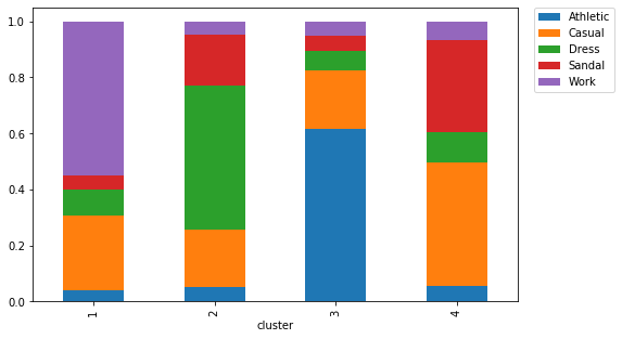
To make sense of the clusters, we build a stacked bar to show the percentage of transactions for a given shoe type made by customers in a given cluster.
[25]:
df_result = df_shoe.merge(df_pivot['cluster'], on='custID').sort_values('transaction')
df_result.pivot_table(values='transaction', index='cluster', columns = ['type'],
                      margins=False, fill_value=0, aggfunc='count')\
            .apply(lambda x: x/x.sum(), axis=1)\
            .plot.bar(stacked=True, figsize=(8,5))
plt.legend(bbox_to_anchor=(1.2, 1), borderaxespad=0)
plt.show()
toggle()
[25]:
The meaning of the clusters is quite apparent. For example, people in cluster 1 tend to buy mostly work shoes, people in cluster 2 tend to buy mostly dress shoes, people in cluster 3 tend to buy mostly athletic shoes, and people in cluster 4 tend to buy mostly sandal or casual shoes.
A First Look on Deep Learning
There is a set of 60,000 training images, plus 10,000 test images, assembled by the National Institute of Standards and Technology (NIST). Each image is a gray scale 28 \(\times\) 28 pixels handwritten digits. we’re trying to classify images into their 10 categories (0 through 9).
[26]:
from keras.datasets import mnist
(train_images, train_labels), (test_images, test_labels) = mnist.load_data()
print('training images:{}, test images:{}'.format(train_images.shape, test_images.shape))
Using TensorFlow backend.
training images:(60000, 28, 28), test images:(10000, 28, 28)
[27]:
def showimg(data, idx):
    span = 5
    if data=='train':
        if idx+span<train_images.shape[0]:
            images = train_images
            labels = train_labels
        else:
            print('Index is out of range.')
    if data=='test':
        if idx+span<test_images.shape[0]:
            images = test_images
            labels = test_labels
        else:
            print('Index is out of range.')
    plt.figure(figsize=(20,4))
    for i in range(span):
        plt.subplot(1, 5, i + 1)
        digit = images[idx+i]
        plt.imshow(digit, cmap=plt.cm.binary)
        plt.title('Index:{}, Label:{}'.format(idx+i, labels[idx+i]), fontsize = 15)
    plt.show()

interact(showimg,
    data = widgets.RadioButtons(options=['train', 'test'],
                                value='train', description='Data:', disabled=False),
    idx = widgets.IntText(value=7, description='Index:', disabled=False));
toggle()
[27]:
Network Architecture
The core building block of neural networks is the layer, a data-processing module working as a filter for data. Specifically, layers extract representations out of the data fed into them in a more useful form which is often called features.
Most of deep learning consists of chaining together simple layers that will implement a form of progressive data distillation. A deep-learning model is like a sieve for data processing, made of a succession of increasingly refined data filters the layers.
network = models.Sequential()
network.add(layers.Dense(512, activation='relu', input_shape=(28 * 28,)))
network.add(layers.Dense(10, activation='softmax'))
Here, our network consists of a sequence of two densely connected (fully connected) layers. The second (and last) layer is a 10-way softmax layer, which means it will return an array of 10 probability scores (summing to 1). Each score will be the probability that the current digit image belongs to one of our 10 digit classes.
Compilation
Before training the network, we need to perform a compilation step by setting up:
An optimizer: the mechanism to improve its performance on the training data
A loss function: the measurement of its performance on the training data
Metrics to monitor during training and testing
network.compile(optimizer='rmsprop',
                loss='categorical_crossentropy',
                metrics=['accuracy'])
Data Preparation
train_images_reshape = train_images.reshape((60000, 28 * 28))
train_images_reshape = train_images_reshape.astype('float32') / 255

test_images_reshape = test_images.reshape((10000, 28 * 28))
test_images_reshape = test_images_reshape.astype('float32') / 255

train_labels_cat = to_categorical(train_labels)
test_labels_cat = to_categorical(test_labels)
Fitting
We train the neural network so that it can classify images in test image set.
network.fit(train_images_reshape, train_labels_cat, epochs=5, batch_size=128)
[28]:
from keras import models
from keras import layers
from keras.utils import to_categorical

network = models.Sequential()
network.add(layers.Dense(512, activation='relu', input_shape=(28 * 28,)))
network.add(layers.Dense(10, activation='softmax'))

network.compile(optimizer='rmsprop',
                loss='categorical_crossentropy',
                metrics=['accuracy'])

train_images_reshape = train_images.reshape((60000, 28 * 28))
train_images_reshape = train_images_reshape.astype('float32') / 255

test_images_reshape = test_images.reshape((10000, 28 * 28))
test_images_reshape = test_images_reshape.astype('float32') / 255

train_labels_cat = to_categorical(train_labels)
test_labels_cat = to_categorical(test_labels)

network.fit(train_images_reshape, train_labels_cat, epochs=5, batch_size=128)

test_loss, test_acc = network.evaluate(test_images_reshape, test_labels_cat)
print('test accuracy:', test_acc)
toggle()
Epoch 1/5
60000/60000 [==============================] - 5s 77us/step - loss: 0.2571 - acc: 0.9263
Epoch 2/5
60000/60000 [==============================] - 4s 62us/step - loss: 0.1039 - acc: 0.9693
Epoch 3/5
60000/60000 [==============================] - 3s 58us/step - loss: 0.0673 - acc: 0.9802
Epoch 4/5
60000/60000 [==============================] - 4s 60us/step - loss: 0.0489 - acc: 0.9850
Epoch 5/5
60000/60000 [==============================] - 4s 63us/step - loss: 0.0368 - acc: 0.9895
10000/10000 [==============================] - 0s 47us/step
test accuracy: 0.9792
[28]:
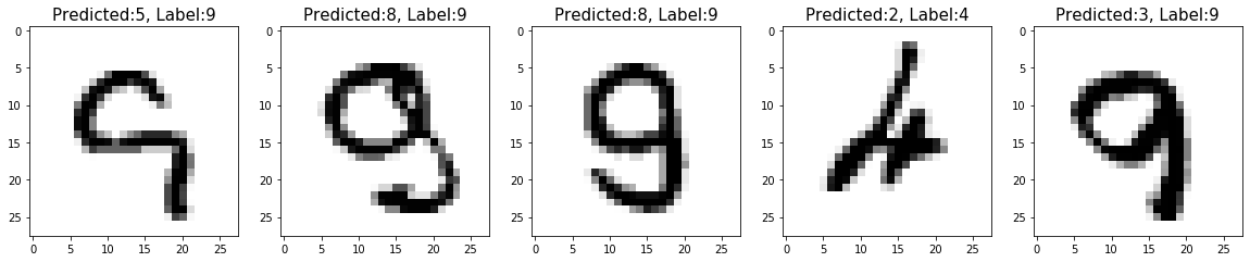
We reach an accuracy of 98.9% on the training data. However, the test-set accuracy turns out to be 97.8% — that’s quite a bit lower than the training set accuracy as our errors are doubled. This gap between training accuracy and test accuracy is an example of overfitting.
Prediction Error
We demonstrate a few images that are misclassified by the trained neural network.
[29]:
predicted = network.predict_classes(test_images_reshape)
result = abs(predicted - test_labels)
misclassified = np.where(result>0)[0]
print('# of misclassified images:',misclassified.shape[0])

plt.figure(figsize=(20,4))
for i in range(5):
    plt.subplot(1, 5, i + 1)
    idx = misclassified[i]
    digit = test_images[idx]
    plt.imshow(digit, cmap=plt.cm.binary)
    plt.title('Predicted:{}, Label:{}'.format(predicted[idx], test_labels[idx]), fontsize = 15)
plt.show()
toggle()
# of misclassified images: 208
[29]:
A Short Introduction to AI

Symbolic AI
Artificial intelligence was proposed by a handful of pioneers from the nascent field of computer science in the 1950s. A concise definition of the field would be as follows: the effort to automate intellectual tasks normally performed by humans.
For a fairly long time, many experts believed that human-level artificial intelligence could be achieved by having programmers handcraft a sufficiently large set of explicit rules for manipulating knowledge. This approach is known as symbolic AI and was the dominant paradigm in AI from the 1950s to the late 1980s.
In the 1960s, people believe that “the problem of creating artificial intelligence will substantially be solved within a generation”. As these high expectations failed to materialize, researchers and government funds turned away from the field, marking the start of the first AI winter.
Expert Systems
In the 1980s, a new take on symbolic AI, expert systems, started gathering steam among large companies. A few initial success stories triggered a wave of investment. Around 1985, companies were spending over $1 billion each year on the technology; but by the early 1990s, these systems had proven expensive to maintain, difficult to scale, and limited in scope, and interest died down. Thus began the second AI winter.
Machine Learning
In classical programming, such as symbolic AI, humans input rules (a program) and data to be processed according to these rules, and out come answers:
\begin{equation} \text{rules $+$ data} \Rightarrow \text{classical programming} \Rightarrow \text{answers} \nonumber \end{equation}
For example, an Expert System contains two main components: an inference engine and a knowledge base.
Expert systems require a real human expert to input knowledge (such as all steps s/he took to make the decision, and how to handle exceptions) into the knowledge base, whereas in machine learning, no such “expert” is needed.
The inference engine applies logical rules based on facts from the knowledge base. These rules are typically in the form of if-then statements. A flexible system would use the knowledge as an initial guide, and use the expert’s guidance to learn, based on feedback from the expert.
Machine learning arises from the question that could a computer go beyond “what we know how to order it to perform” and learn on its own how to perform a specified task? A machine-learning system is trained rather than explicitly programmed. The programming paradigm is quite different
\begin{equation} \text{data $+$ answers} \Rightarrow \text{machine learning} \Rightarrow \text{rules} \nonumber \end{equation}
Machine learning is a type of artificial intelligence. It can be broadly divided into supervised, unsupervised, self-supervised and reinforcement learning.
In supervised learning, a computer is given a set of data and an expected result, and asked to find relationships between the data and the result. The computer can then learn how to predict the result when given new data. It’s by far the dominant form of deep learning today.
In unsupervised learning, a computer has data to play with but no expected result. It is asked to find relationships between entries in the dataset to discover new patterns.
Self-supervised learning is supervised learning without human-annotated labels such as autoencoders.
In reinforcement learning, an agent receives information about its environment and learns to choose actions that will maximize some reward. Currently, reinforcement learning is mostly a research area and hasn’t yet had significant practical successes beyond games.
Machine learning started to flourish in the 1990s and has quickly become the most popular and most successful subfield of AI.
Deep Learning
Deep learning is a specific subfield of machine learning: a new take on learning information from data that puts an emphasis on learning successive layers of increasingly meaningful representations.
The “deep” in deep learning
it isn’t a reference to any kind of deeper understanding achieved by the approach;
it stands for the idea of successive layers of representations.
Shallow learning is referring to approaches in machine learning that focus on learning only one or two layers of representations of the data.
See the deep representations learned by a 4-layer neural network for digit number 4.

Is deep learning an AI Hype?
Although some world-changing applications like autonomous cars are already within reach, many more are likely to remain elusive for a long time, such as believable dialogue systems, human-level machine translation across arbitrary languages, and human-level natural-language understanding. In particular, talk of human-level general intelligence shouldn’t be taken too seriously. The risk with high expectations for the short term is that, as technology fails to deliver, research investment will dry up, slowing progress for a long time.
Although we’re still in the phase of intense optimism, we may be currently witnessing the third cycle of AI hype and disappointment.
The Promise
Although we may have unrealistic short-term expectations for AI, the long-term picture is looking bright. We’re only getting started in applying deep learning in real-world applications. Right now, it may seem hard to believe that AI could have a large impact on our world, because it isn’t yet widely deployed — much as, back in 1995, it would have been difficult to believe in the future impact of the internet.
Don’t believe the short-term hype, but do believe in the long-term vision. Deep learning has several properties that justify its status as an AI revolution:
Simplicity: Deep learning removes the need for many heavy-duty engineering preprocessing.
Scalability: Deep learning is highly amenable to parallelization on GPUs or TPUs. Deep-learning models are trained by iterating over small batches of data, allowing them to be trained on datasets of pretty much arbitrary size.
Versatility and reusability: deep-learning models can be trained on additional data without restarting from scratch. Trained deep-learning models are repurposable. For instance, it’s possible to take a deep-learning model trained for image classification and drop it into a video processing pipeline.
Deep learning has only been in the spotlight for a few years, and we haven’t yet established the full scope of what it can do.
Neural Network Structures
Tensors are fundamental to the data representations for neural networks — so fundamental that Google’s TensorFlow was named after them.

Scalars: 0 dimensional tensors
Vectors: 1 dimensional tensors
Matrix: 2 dimensional tensors
Let’s make data tensors more concrete with real-world examples:
Vector data — 2D tensors of shape (samples, features)
Timeseries data or sequence data — 3D tensors of shape (samples, timesteps, features)
Images — 4D tensors of shape (samples, height, width, channels) or (samples, channels, height, width)
Video — 5D tensors of shape (samples, frames, height, width, channels) or (samples, frames, channels, height, width)
There are mainly three families of network architectures that are densely connected networks, convolutional networks, and recurrent networks. A network architecture encodes assumptions about the structure of the data.
A densely connected network is a stack of Dense layers and assume no specific structure in the input features.
Convnets, or convolutional networks (CNNs), consist of stacks of convolution and max-pooling layers. Convolution layers look at spatially local patterns by applying the same geometric transformation to different spatial locations (patches) in an input tensor.
Recurrent neural networks (RNNs) work by processing sequences of inputs one time step at a time and maintaining a state throughout
Prediction v.s. Decision
What is the capital of Delaware?
[30]:
hide_answer()
[30]:
A machine called Alexa says the correct answer: “The capital of Delaware is Dover.”
The new wave of artificial intelligence does not actually bring us intelligence but instead a critical component of intelligence — prediction.
What Alexa was doing when we asked a question was taking the sounds it heard and predicting the words we spoke and then predicting what information the words were looking for.
Alexa doesn’t “know” the capital of Delaware. But Alexa is able to predict that, when people ask such a question, they are looking for a specific response: Dover.
\(\blacksquare\)
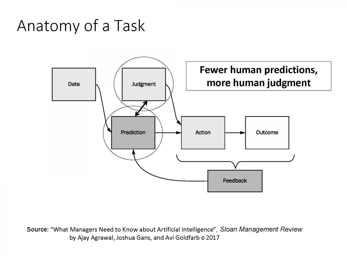
What is the difference between judgment and prediction?
[31]:
hide_answer()
[31]:

In the movie “I, Robot.”, there’s one scene that makes it very clear what this distinction between prediction and judgment is.
Will Smith is the star of the movie and he has a flashback scene where he’s in a car accident with a 12-year-old girl. And they’re drowning and then a robot arrives, somehow miraculously, and can save one of them.
The robot apparently makes this calculation that Will Smith has a 45% chance of survival and the girl only had an 11% chance. And therefore, the robot saves Will Smith.
Will Smith concludes that the robot made the wrong decision. 11% was more than enough. A human being would have known that.
So that’s all well and good and he’s assuming that the robot values his life and the girl’s life the same. But in order for the robot to make a decision, it needs the prediction on survival and a statement about how much more valuable the girl’s life has to be than Will Smith’s life in order to choose.
This decision that we’ve seen, all it says is Will Smith’s life is worth at least a quarter of the girl’s life. That valuation decision matters, because at some point even Will Smith would disagree with this. At some point, if her chance of survival was 1%, or 0.1%, or 0.01%, that decision would flip. That’s judgment. That’s knowing what to do with the prediction once you have one.
So judgment is the process of determining what the reward is to a particular action in a particular environment. Decision analysis tools (such as optimization and simulation) can be used for balancing the reward and cost (or risk).
We need to understand the consequences of cheap prediction and its importance in decision-making
\(\blacksquare\)
Current Status of Deep Learning
Achievements
Deep learning has achieved the following breakthroughs, all in historically difficult areas of machine learning:
Near-human-level image classification
Near-human-level speech recognition
Near-human-level handwriting transcription
Improved machine translation
Improved text-to-speech conversion
Digital assistants such as Google Now and Amazon Alexa
Near-human-level autonomous driving
Improved ad targeting, as used by Google, Baidu, and Bing
Improved search results on the web
Ability to answer natural-language questions
Superhuman Go playing
Hardware
Although our laptop can run small deep-learning models, typical deep-learning models used in computer vision or speech recognition require orders of magnitude more computational power.
Throughout the 2000s, companies like NVIDIA and AMD have been investing billions of dollars in developing fast, massively parallel chips, graphical processing units (GPUs), to power the graphics of increasingly photorealistic video games — cheap, single-purpose supercomputers designed to render complex 3D scenes on the screen in real time.
At the end of 2015, the NVIDIA TITAN X, a gaming GPU that cost $1,000 can perform 6.6 trillion float32 operations per second. That is about 350 times more than what you can get out of a modern laptop. Meanwhile, large companies train deep-learning models on clusters of hundreds of GPUs of a type developed specifically for the needs of deep learning, such as the NVIDIA Tesla K80. The sheer computational power of such clusters is something that would never have been possible without modern
GPUs.
The deep-learning industry is starting to go beyond GPUs and is investing in increasingly specialized, efficient chips for deep learning. In 2016, at its annual I/O convention, Google revealed its tensor processing unit (TPU) project: a new chip design developed from the ground up to run deep neural networks, which is reportedly 10 times faster and far more energy efficient than top-of-the-line GPUs.
If you don’t already have a GPU that you can use for deep learning, then running deep-learning experiments in the cloud is a simple, low cost way for you to get started without having to buy any additional hardware. But if you’re a heavy user of deep learning, this setup isn’t sustainable in the long term or even for more than a few weeks.
Investment
As deep learning became the new state of the art for computer vision and eventually for all perceptual tasks, industry leaders took note. What followed was a gradual wave of industry investment far beyond anything previously seen in the history of AI.
In 2011 (right before deep learning took the spotlight), the total venture capital investment in AI was around $19 million
By 2014, the total venture capital investment in AI had risen to $394 million
Google acquired the deep-learning startup DeepMind for a reported $500 million — the largest acquisition of an AI company in history.
Baidu started a deep-learning research center in Silicon Valley, investing $300 million in the project.
Intel acquired a deep-learning hardware startup Nervana Systems for over $400 million.
There are currently no signs that this uptrend will slow any time soon.
As entrepreneurs of AI start-ups, Alice and Bob had received similar amount of investments and competed in the same market
Alice spent lots of money to hire top engineers in AI field
Bob hired only mediocre engineers and spent most of his money to obtain high quality data with larger size
Who will you invest? Why?
[32]:
hide_answer()
[32]:
acc1 = net_compare(512, .25)
acc2 = net_compare(128, 1)
print('The accuracy of a complicated model (with 512 nodes) with less (one fourth of) training data:', acc1)
print('The accuracy of a simple model (with 128 nodes) and full training data:', acc2)
print('The improvement is {}%!'.format(round((acc2-acc1)/(1-acc1)*100,2)))
\(\blacksquare\)
Development
Suppose you’re trying to develop a model that can take as input images of a clock

and can output the time of day. What machine learning approach will you use?
[33]:
hide_answer()
[33]:
If you choose to use the raw pixels of the image as input data, then you have a difficult machine-learning problem on your hands. You’ll need a convolutional neural network to solve it, and you’ll have to expend quite a bit of computational resources to train the network.
But if you already understand the problem at a high level, you can write a five-line Python script to follow the black pixels of the clock hands and output the \((x, y)\) coordinates of the tip of each hand.
Then a simple machine-learning algorithm can learn to associate these coordinates with the appropriate time of day. For example,
the long hand has \((x=0.7, y=0.7)\) and the short hand has \((x=0.5, y=0.0)\) in the first image, and
the long hand has \((x=0.0, y=1.0)\) and the short hand has \((x=-0.38, y=0.32)\) in the second image.
You can go even further: do a coordinate change, and express the \((x, y)\) coordinates as the angle of each clock hand. For example,
the long hand has angle \(45\) degree and the short hand has angle \(0\) degree in the first image, and
the long hand has angle \(90\) degree and the short hand has angle \(140\) degree in the second image.
At this point, your features are making the problem so easy that no machine learning is required; a simple rounding operation and dictionary lookup are enough to recover the approximate time of day.
\(\blacksquare\)