[1]:
%run ../initscript.py
HTML("""
<div id="popup" style="padding-bottom:5px; display:none;">
    <div>Enter Password:</div>
    <input id="password" type="password"/>
    <button onclick="done()" style="border-radius: 12px;">Submit</button>
</div>
<button onclick="unlock()" style="border-radius: 12px;">Unclock</button>
<a href="#" onclick="code_toggle(this); return false;">show code</a>
""")
[1]:
[2]:
%run loadregfuncs.py

from ipywidgets import *
import warnings
warnings.filterwarnings('ignore')
warnings.simplefilter('ignore')
%matplotlib inline

toggle()
[2]:
Regression Modeling
Categorical Variables
The only meaningful way to summarize categorical data is with counts of observations in the categories. We consider a bank’s employee data.
[3]:
df_salary = pd.read_csv(dataurl+'salaries.csv', header=0, index_col='employee')
interact(plot_hist,
         column=widgets.Dropdown(options=df_salary.columns[:-1],value=df_salary.columns[0],
                            description='Column:',disabled=False));
To analyze whether the bank discriminates against females in terms of salary, we consider regression model:
[4]:
df = pd.read_csv(dataurl+'salaries.csv', header=0, index_col='employee')
result = analysis(df, 'salary', ['years1', 'years2', 'C(gender, Treatment(\'Male\'))'], printlvl=5)
| Dep. Variable: | salary | R-squared: | 0.492 |
|---|---|---|---|
| Model: | OLS | Adj. R-squared: | 0.485 |
| Method: | Least Squares | F-statistic: | 65.93 |
| Date: | Mon, 20 May 2019 | Prob (F-statistic): | 7.61e-30 |
| Time: | 13:53:58 | Log-Likelihood: | -2164.5 |
| No. Observations: | 208 | AIC: | 4337. |
| Df Residuals: | 204 | BIC: | 4350. |
| Df Model: | 3 | ||
| Covariance Type: | nonrobust |
| coef | std err | t | P>|t| | [0.025 | 0.975] | |
|---|---|---|---|---|---|---|
| Intercept | 3.549e+04 | 1341.022 | 26.466 | 0.000 | 3.28e+04 | 3.81e+04 |
| C(gender, Treatment('Male'))[T.Female] | -8080.2121 | 1198.170 | -6.744 | 0.000 | -1.04e+04 | -5717.827 |
| years1 | 987.9937 | 80.928 | 12.208 | 0.000 | 828.431 | 1147.557 |
| years2 | 131.3379 | 180.923 | 0.726 | 0.469 | -225.381 | 488.057 |
| Omnibus: | 15.654 | Durbin-Watson: | 1.286 |
|---|---|---|---|
| Prob(Omnibus): | 0.000 | Jarque-Bera (JB): | 25.154 |
| Skew: | 0.434 | Prob(JB): | 3.45e-06 |
| Kurtosis: | 4.465 | Cond. No. | 34.6 |
Warnings:
[1] Standard Errors assume that the covariance matrix of the errors is correctly specified.
standard error of estimate:8079.39743


ANOVA Table:
| sum_sq | df | F | PR(>F) | |
|---|---|---|---|---|
| C(gender, Treatment('Male')) | 2.968701e+09 | 1.0 | 45.478753 | 1.556196e-10 |
| years1 | 9.728975e+09 | 1.0 | 149.042170 | 4.314965e-26 |
| years2 | 3.439940e+07 | 1.0 | 0.526979 | 4.687119e-01 |
| Residual | 1.331644e+10 | 204.0 | NaN | NaN |
The regression is equivalent to fit data into two separate regression functions. However, it is usually easier and more efficient to answer research questions concerning the binary predictor variable by using one combined regression function.
[5]:
def update(column):
    df = pd.read_csv(dataurl+'salaries.csv', header=0, index_col='employee')
    sns.lmplot(x=column, y='salary', data=df, fit_reg=True, hue='gender', legend=True, height=6);

interact(update,
         column=widgets.Dropdown(options=['years1', 'years2', 'age', 'education'],value='years1',
                            description='Column:',disabled=False));
Interaction Variables
Interaction with Categorical Variable
Example: consider salary data with interaction gender*year1
[6]:
result = ols(formula="salary ~ years1 + C(gender, Treatment('Male'))*years1", data=df_salary).fit()
display(result.summary())
print("\nANOVA Table:\n")
display(sm.stats.anova_lm(result, typ=1))
| Dep. Variable: | salary | R-squared: | 0.639 |
|---|---|---|---|
| Model: | OLS | Adj. R-squared: | 0.633 |
| Method: | Least Squares | F-statistic: | 120.2 |
| Date: | Mon, 20 May 2019 | Prob (F-statistic): | 7.51e-45 |
| Time: | 13:54:00 | Log-Likelihood: | -2129.2 |
| No. Observations: | 208 | AIC: | 4266. |
| Df Residuals: | 204 | BIC: | 4280. |
| Df Model: | 3 | ||
| Covariance Type: | nonrobust |
| coef | std err | t | P>|t| | [0.025 | 0.975] | |
|---|---|---|---|---|---|---|
| Intercept | 3.043e+04 | 1216.574 | 25.013 | 0.000 | 2.8e+04 | 3.28e+04 |
| C(gender, Treatment('Male'))[T.Female] | 4098.2519 | 1665.842 | 2.460 | 0.015 | 813.776 | 7382.727 |
| years1 | 1527.7617 | 90.460 | 16.889 | 0.000 | 1349.405 | 1706.119 |
| C(gender, Treatment('Male'))[T.Female]:years1 | -1247.7984 | 136.676 | -9.130 | 0.000 | -1517.277 | -978.320 |
| Omnibus: | 11.523 | Durbin-Watson: | 1.188 |
|---|---|---|---|
| Prob(Omnibus): | 0.003 | Jarque-Bera (JB): | 15.614 |
| Skew: | 0.379 | Prob(JB): | 0.000407 |
| Kurtosis: | 4.108 | Cond. No. | 58.3 |
Warnings:
[1] Standard Errors assume that the covariance matrix of the errors is correctly specified.
ANOVA Table:
| df | sum_sq | mean_sq | F | PR(>F) | |
|---|---|---|---|---|---|
| C(gender, Treatment('Male')) | 1.0 | 3.149634e+09 | 3.149634e+09 | 67.789572 | 2.150454e-14 |
| years1 | 1.0 | 9.726635e+09 | 9.726635e+09 | 209.346370 | 4.078705e-33 |
| C(gender, Treatment('Male')):years1 | 1.0 | 3.872606e+09 | 3.872606e+09 | 83.350112 | 6.833545e-17 |
| Residual | 204.0 | 9.478232e+09 | 4.646192e+07 | NaN | NaN |
Example: Let’s consider some contrived data
[7]:
np.random.seed(123)
size = 20
x1 = np.linspace(-5,5,size)
group = np.random.randint(0, 2, size=size)
y = 5 + (3-7*group)*x1 + 3*np.random.normal(size=size)
df = pd.DataFrame({'y':y, 'x1':x1, 'group':group})
sns.lmplot(x='x1', y='y', data=df, fit_reg=True, hue='group', legend=True);
result = analysis(df, 'y', ['x1', 'group'], printlvl=4)
| Dep. Variable: | y | R-squared: | 0.004 |
|---|---|---|---|
| Model: | OLS | Adj. R-squared: | -0.113 |
| Method: | Least Squares | F-statistic: | 0.03659 |
| Date: | Mon, 20 May 2019 | Prob (F-statistic): | 0.964 |
| Time: | 13:54:00 | Log-Likelihood: | -72.898 |
| No. Observations: | 20 | AIC: | 151.8 |
| Df Residuals: | 17 | BIC: | 154.8 |
| Df Model: | 2 | ||
| Covariance Type: | nonrobust |
| coef | std err | t | P>|t| | [0.025 | 0.975] | |
|---|---|---|---|---|---|---|
| Intercept | 3.1116 | 3.075 | 1.012 | 0.326 | -3.377 | 9.600 |
| x1 | 0.1969 | 0.765 | 0.257 | 0.800 | -1.417 | 1.811 |
| group | 0.0733 | 4.667 | 0.016 | 0.988 | -9.773 | 9.920 |
| Omnibus: | 0.957 | Durbin-Watson: | 2.131 |
|---|---|---|---|
| Prob(Omnibus): | 0.620 | Jarque-Bera (JB): | 0.741 |
| Skew: | 0.008 | Prob(JB): | 0.690 |
| Kurtosis: | 2.057 | Cond. No. | 7.06 |
Warnings:
[1] Standard Errors assume that the covariance matrix of the errors is correctly specified.
standard error of estimate:10.04661
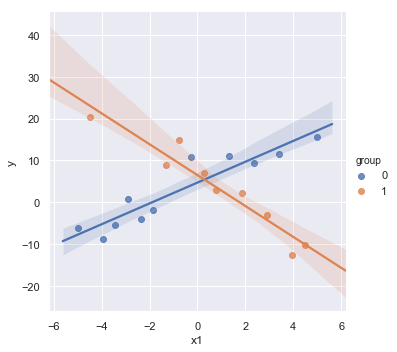
The scatterplot shows that both explanatory variables x and group are related to y. However, the regression results show that there is insufficient evidence to conclude that x and group are related to y. The example shows that if we leave an important interaction term out of our model, our analysis can lead us to make erroneous conclusions.
Without interaction variables, we assume the effect of each \(X\) on \(Y\) is independent of the value of the other \(X\)’s, which is not the case in this contrived data as shown in the scatterplot.
Now, consider a regression model contains an interaction term between the two predictors.
[8]:
result = analysis(df, 'y', ['x1', 'x1*C(group)'], printlvl=4)
| Dep. Variable: | y | R-squared: | 0.897 |
|---|---|---|---|
| Model: | OLS | Adj. R-squared: | 0.878 |
| Method: | Least Squares | F-statistic: | 46.57 |
| Date: | Mon, 20 May 2019 | Prob (F-statistic): | 3.95e-08 |
| Time: | 13:54:01 | Log-Likelihood: | -50.187 |
| No. Observations: | 20 | AIC: | 108.4 |
| Df Residuals: | 16 | BIC: | 112.4 |
| Df Model: | 3 | ||
| Covariance Type: | nonrobust |
| coef | std err | t | P>|t| | [0.025 | 0.975] | |
|---|---|---|---|---|---|---|
| Intercept | 4.7029 | 1.027 | 4.578 | 0.000 | 2.525 | 6.881 |
| C(group)[T.1] | 1.7810 | 1.552 | 1.147 | 0.268 | -1.509 | 5.071 |
| x1 | 2.4905 | 0.319 | 7.798 | 0.000 | 1.813 | 3.168 |
| x1:C(group)[T.1] | -6.1842 | 0.524 | -11.792 | 0.000 | -7.296 | -5.072 |
| Omnibus: | 1.739 | Durbin-Watson: | 1.433 |
|---|---|---|---|
| Prob(Omnibus): | 0.419 | Jarque-Bera (JB): | 1.403 |
| Skew: | 0.607 | Prob(JB): | 0.496 |
| Kurtosis: | 2.541 | Cond. No. | 7.68 |
Warnings:
[1] Standard Errors assume that the covariance matrix of the errors is correctly specified.
standard error of estimate:3.32671
The non-significance for the coefficients of group indicates no observed difference between the mean values of x1 in different groups.
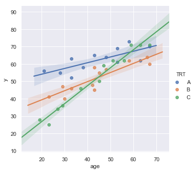
Example: Researchers are interested in comparing the effectiveness of three treatments (A,B,C) for severe depression. They collect the data on a random sample of \(n = 36\) severely depressed individuals including following variables:
measure of the effectiveness of the treatment for each individual
age (in years) of each individual i
x2 = 1 if an individual is received treatment A and 0, if not
x3 = 1 if an individual is received treatment B and 0, if not
The regression model:
\begin{align} \text{y} = \beta_0 + \beta_1 \times \text{age} + \beta_2 \times \text{x2} + \beta_3 \times \text{x3} + \beta_{12} \times \text{age} \times \text{x2} + \beta_{13} \times \text{age} \times \text{x3} \end{align}
[9]:
df = pd.read_csv(dataurl+'depression.txt', delim_whitespace=True, header=0)
sns.lmplot(x='age', y='y', data=df, fit_reg=True, hue='TRT', legend=True);
[10]:
result = analysis(df, 'y', ['age', 'age*x2', 'age*x3'], printlvl=4)
sm.stats.anova_lm(result, typ=1)
| Dep. Variable: | y | R-squared: | 0.914 |
|---|---|---|---|
| Model: | OLS | Adj. R-squared: | 0.900 |
| Method: | Least Squares | F-statistic: | 64.04 |
| Date: | Mon, 20 May 2019 | Prob (F-statistic): | 4.26e-15 |
| Time: | 13:54:03 | Log-Likelihood: | -97.024 |
| No. Observations: | 36 | AIC: | 206.0 |
| Df Residuals: | 30 | BIC: | 215.5 |
| Df Model: | 5 | ||
| Covariance Type: | nonrobust |
| coef | std err | t | P>|t| | [0.025 | 0.975] | |
|---|---|---|---|---|---|---|
| Intercept | 6.2114 | 3.350 | 1.854 | 0.074 | -0.630 | 13.052 |
| age | 1.0334 | 0.072 | 14.288 | 0.000 | 0.886 | 1.181 |
| x2 | 41.3042 | 5.085 | 8.124 | 0.000 | 30.920 | 51.688 |
| age:x2 | -0.7029 | 0.109 | -6.451 | 0.000 | -0.925 | -0.480 |
| x3 | 22.7068 | 5.091 | 4.460 | 0.000 | 12.310 | 33.104 |
| age:x3 | -0.5097 | 0.110 | -4.617 | 0.000 | -0.735 | -0.284 |
| Omnibus: | 2.593 | Durbin-Watson: | 1.633 |
|---|---|---|---|
| Prob(Omnibus): | 0.273 | Jarque-Bera (JB): | 1.475 |
| Skew: | -0.183 | Prob(JB): | 0.478 |
| Kurtosis: | 2.079 | Cond. No. | 529. |
Warnings:
[1] Standard Errors assume that the covariance matrix of the errors is correctly specified.
standard error of estimate:3.92491
[10]:
| df | sum_sq | mean_sq | F | PR(>F) | |
|---|---|---|---|---|---|
| age | 1.0 | 3424.431786 | 3424.431786 | 222.294615 | 2.058902e-15 |
| x2 | 1.0 | 803.804498 | 803.804498 | 52.178412 | 4.856763e-08 |
| age:x2 | 1.0 | 375.254832 | 375.254832 | 24.359407 | 2.794727e-05 |
| x3 | 1.0 | 0.936671 | 0.936671 | 0.060803 | 8.069102e-01 |
| age:x3 | 1.0 | 328.424475 | 328.424475 | 21.319447 | 6.849515e-05 |
| Residual | 30.0 | 462.147738 | 15.404925 | NaN | NaN |
For each age, is there a difference in the mean effectiveness for the three treatments?
[11]:
hide_answer()
[11]:
\begin{align*} \text{Treatment A:} & \quad \mu_Y = (\beta_0 + \beta_2) + (\beta_1 + \beta_{12}) \times \text{age} \\ \text{Treatment B:} & \quad \mu_Y = (\beta_0 + \beta_3) + (\beta_1 + \beta_{13}) \times \text{age} \\ \text{Treatment C:} & \quad \mu_Y = \beta_0 + \beta_1 \times \text{age} \end{align*}
The research question is equivalent to ask \begin{align*} \text{Treatment A} - \text{Treatment C} &= 0 = \beta_2 + \beta_{12} \times \text{age} \\ \text{Treatment B} - \text{Treatment C} &= 0 = \beta_3 + \beta_{13} \times \text{age} \end{align*}
Thus, we test hypothesis \begin{align} H_0:& \quad \beta_2 = \beta_3 = \beta_{12} = \beta_{13} = 0 \nonumber\\ H_a:& \quad \text{at least one is nonzero} \nonumber \end{align}
The python code is:
_ =GL_Ftest(df, 'y', ['age', 'x2', 'x3', 'age:x2', 'age:x3'], ['age'], 0.05, typ=1)
Does the effect of age on the treatment’s effectiveness depend on treatment?
[12]:
hide_answer()
[12]:
The question asks if the two interaction parameters \(\beta_{12}\) and \(\beta_{13}\) are significant.
The python code is:
_ =GL_Ftest(df, 'y', ['age', 'x2', 'x3', 'age:x2', 'age:x3'], ['age', 'x2', 'x3'], 0.05, typ=1)
Interactions Between Continuous Variables
Typically, regression models that include interactions between quantitative predictors adhere to the hierarchy principle, which says that if your model includes an interaction term, \(X_1 X_2\), and \(X_1 X_2\) is shown to be a statistically significant predictor of Y, then your model should also include the “main effects,” \(X_1\) and \(X_2\), whether or not the coefficients for these main effects are significant. Depending on the subject area, there may be circumstances where a main effect could be excluded, but this tends to be the exception.
Transformations
Log-transform
Transformation is used widely in regression analysis because they have a meaningful interpretation.
\(Y = a \log(X) + \cdots\): 1% increase by X, Y is expected to increase by 0.01*a amount
\(\log(Y) = a X + \cdots\): 1unit increase by X, Y is expected to increase by (100*a)%
\(\log(Y) = a \log(X) + \cdots\): 1% increase by X, Y is expected to increase by a%
Transforming the \(X\) values is appropriate when non-linearity is the only problem (i.e., the independence, normality, and equal variance conditions are met)
Transforming the \(Y\) values should be considered when non-normality and/or unequal variances are the problems with the model.
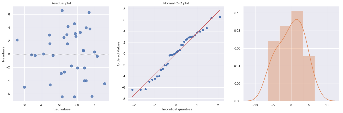
[13]:
df = pd.read_csv(dataurl+'shortleaf.txt', delim_whitespace=True, header=0)
result = analysis(df, 'Vol', ['Diam'], printlvl=4)
| Dep. Variable: | Vol | R-squared: | 0.893 |
|---|---|---|---|
| Model: | OLS | Adj. R-squared: | 0.891 |
| Method: | Least Squares | F-statistic: | 564.9 |
| Date: | Mon, 20 May 2019 | Prob (F-statistic): | 1.17e-34 |
| Time: | 13:54:11 | Log-Likelihood: | -258.61 |
| No. Observations: | 70 | AIC: | 521.2 |
| Df Residuals: | 68 | BIC: | 525.7 |
| Df Model: | 1 | ||
| Covariance Type: | nonrobust |
| coef | std err | t | P>|t| | [0.025 | 0.975] | |
|---|---|---|---|---|---|---|
| Intercept | -41.5681 | 3.427 | -12.130 | 0.000 | -48.406 | -34.730 |
| Diam | 6.8367 | 0.288 | 23.767 | 0.000 | 6.263 | 7.411 |
| Omnibus: | 29.509 | Durbin-Watson: | 0.562 |
|---|---|---|---|
| Prob(Omnibus): | 0.000 | Jarque-Bera (JB): | 85.141 |
| Skew: | 1.240 | Prob(JB): | 3.25e-19 |
| Kurtosis: | 7.800 | Cond. No. | 34.8 |
Warnings:
[1] Standard Errors assume that the covariance matrix of the errors is correctly specified.
standard error of estimate:9.87485
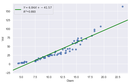
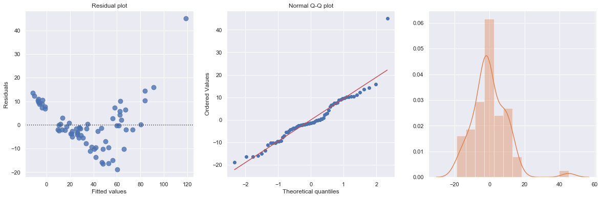
The Q-Q plot suggests that the error terms are not normal. We can log-transform \(X\) (Diam).
[14]:
df = pd.read_csv(dataurl+'shortleaf.txt', delim_whitespace=True, header=0)
df['logvol'] = np.log(df.Vol)
df['logdiam'] = np.log(df.Diam)
result = analysis(df, 'Vol', ['logdiam'], printlvl=4)
| Dep. Variable: | Vol | R-squared: | 0.746 |
|---|---|---|---|
| Model: | OLS | Adj. R-squared: | 0.743 |
| Method: | Least Squares | F-statistic: | 200.2 |
| Date: | Mon, 20 May 2019 | Prob (F-statistic): | 6.10e-22 |
| Time: | 13:54:14 | Log-Likelihood: | -288.66 |
| No. Observations: | 70 | AIC: | 581.3 |
| Df Residuals: | 68 | BIC: | 585.8 |
| Df Model: | 1 | ||
| Covariance Type: | nonrobust |
| coef | std err | t | P>|t| | [0.025 | 0.975] | |
|---|---|---|---|---|---|---|
| Intercept | -116.1618 | 10.830 | -10.726 | 0.000 | -137.773 | -94.551 |
| logdiam | 64.5358 | 4.562 | 14.148 | 0.000 | 55.433 | 73.638 |
| Omnibus: | 50.047 | Durbin-Watson: | 0.324 |
|---|---|---|---|
| Prob(Omnibus): | 0.000 | Jarque-Bera (JB): | 219.500 |
| Skew: | 2.099 | Prob(JB): | 2.17e-48 |
| Kurtosis: | 10.591 | Cond. No. | 16.6 |
Warnings:
[1] Standard Errors assume that the covariance matrix of the errors is correctly specified.
standard error of estimate:15.17022
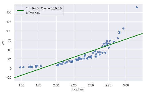
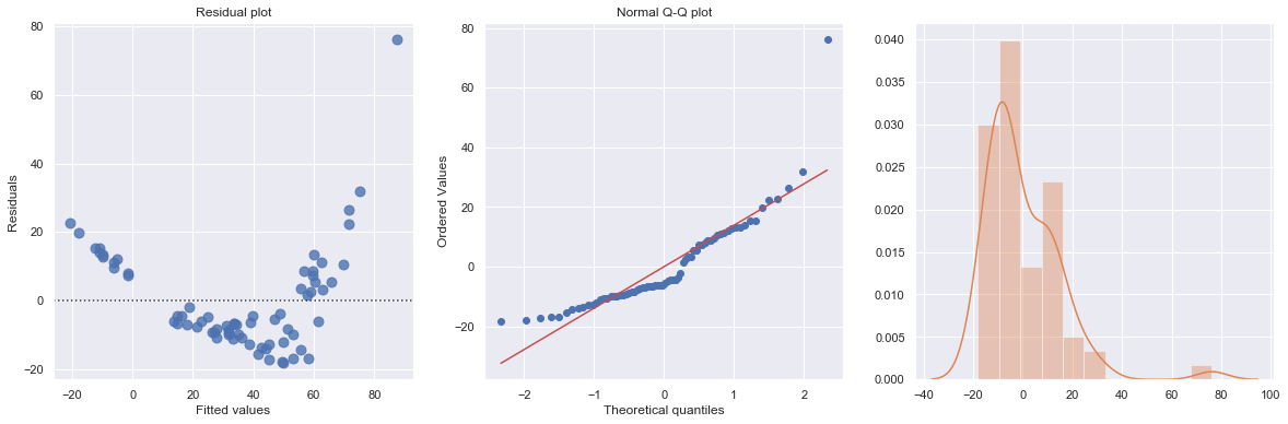
Transforming only the x values doesn’t change the non-linearity at all and improve the normality of the error terms either. We perform log-transform on both \(X\) and \(Y\).
[15]:
result = analysis(df, 'logvol', ['logdiam'], printlvl=4)
| Dep. Variable: | logvol | R-squared: | 0.974 |
|---|---|---|---|
| Model: | OLS | Adj. R-squared: | 0.973 |
| Method: | Least Squares | F-statistic: | 2509. |
| Date: | Mon, 20 May 2019 | Prob (F-statistic): | 2.08e-55 |
| Time: | 13:54:14 | Log-Likelihood: | 25.618 |
| No. Observations: | 70 | AIC: | -47.24 |
| Df Residuals: | 68 | BIC: | -42.74 |
| Df Model: | 1 | ||
| Covariance Type: | nonrobust |
| coef | std err | t | P>|t| | [0.025 | 0.975] | |
|---|---|---|---|---|---|---|
| Intercept | -2.8718 | 0.122 | -23.626 | 0.000 | -3.114 | -2.629 |
| logdiam | 2.5644 | 0.051 | 50.090 | 0.000 | 2.462 | 2.667 |
| Omnibus: | 1.405 | Durbin-Watson: | 1.359 |
|---|---|---|---|
| Prob(Omnibus): | 0.495 | Jarque-Bera (JB): | 1.119 |
| Skew: | -0.051 | Prob(JB): | 0.572 |
| Kurtosis: | 2.389 | Cond. No. | 16.6 |
Warnings:
[1] Standard Errors assume that the covariance matrix of the errors is correctly specified.
standard error of estimate:0.17026
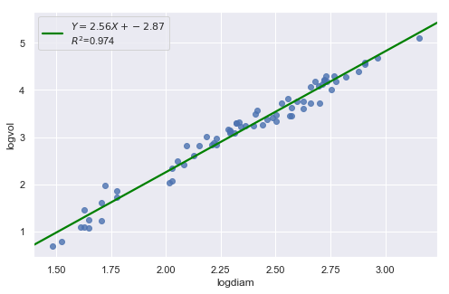
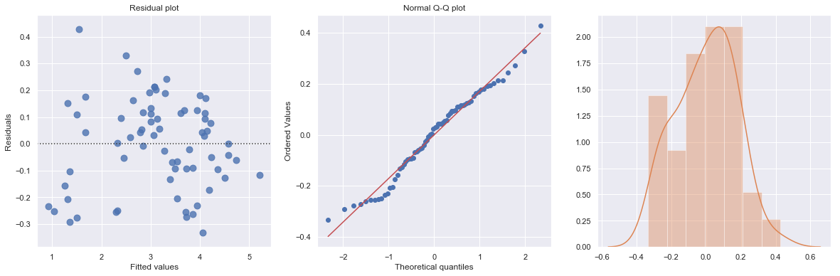
The residual and Q-Q plot has improved substantially
Polynomial Transformations
[16]:
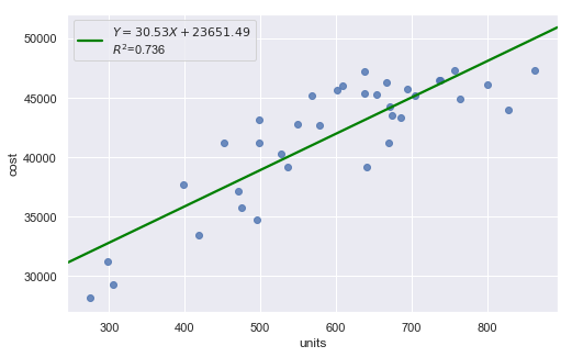
df = pd.read_csv(dataurl+'costunits.csv', header=0, index_col='month')
result = analysis(df, 'cost', ['units'], printlvl=4)
| Dep. Variable: | cost | R-squared: | 0.736 |
|---|---|---|---|
| Model: | OLS | Adj. R-squared: | 0.728 |
| Method: | Least Squares | F-statistic: | 94.75 |
| Date: | Mon, 20 May 2019 | Prob (F-statistic): | 2.32e-11 |
| Time: | 13:54:15 | Log-Likelihood: | -334.94 |
| No. Observations: | 36 | AIC: | 673.9 |
| Df Residuals: | 34 | BIC: | 677.0 |
| Df Model: | 1 | ||
| Covariance Type: | nonrobust |
| coef | std err | t | P>|t| | [0.025 | 0.975] | |
|---|---|---|---|---|---|---|
| Intercept | 2.365e+04 | 1917.137 | 12.337 | 0.000 | 1.98e+04 | 2.75e+04 |
| units | 30.5331 | 3.137 | 9.734 | 0.000 | 24.158 | 36.908 |
| Omnibus: | 4.527 | Durbin-Watson: | 2.144 |
|---|---|---|---|
| Prob(Omnibus): | 0.104 | Jarque-Bera (JB): | 1.765 |
| Skew: | -0.042 | Prob(JB): | 0.414 |
| Kurtosis: | 1.918 | Cond. No. | 2.57e+03 |
Warnings:
[1] Standard Errors assume that the covariance matrix of the errors is correctly specified.
[2] The condition number is large, 2.57e+03. This might indicate that there are
strong multicollinearity or other numerical problems.
standard error of estimate:2733.74240
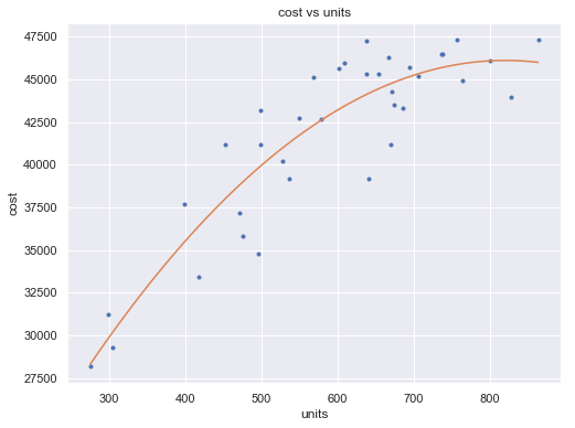
[17]:
df = pd.read_csv(dataurl+'costunits.csv', header=0, index_col='month')
fit2 = np.poly1d(np.polyfit(df.units, df.cost, 2))
xp = np.linspace(np.min(df.units), np.max(df.units), 100)
fig = plt.figure(figsize=(8,6))
plt.plot(df.units, df.cost, '.', xp, fit2(xp), '-')
plt.title('cost vs units')
plt.xlabel('units')
plt.ylabel('cost')
plt.show()

toggle()
[17]:
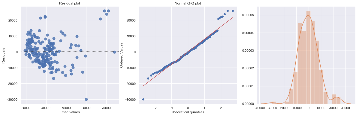
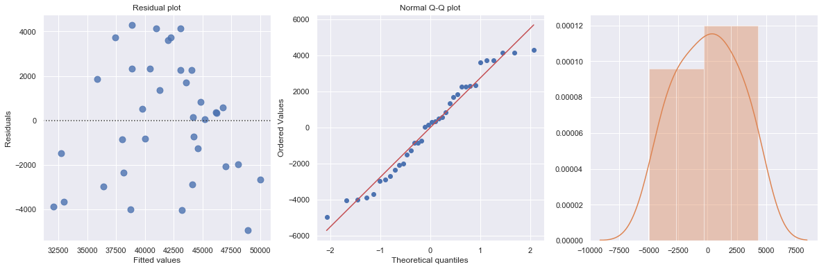
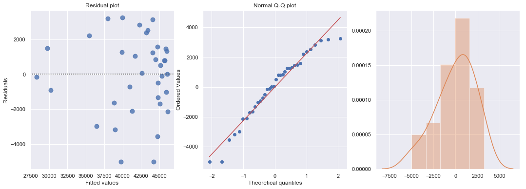
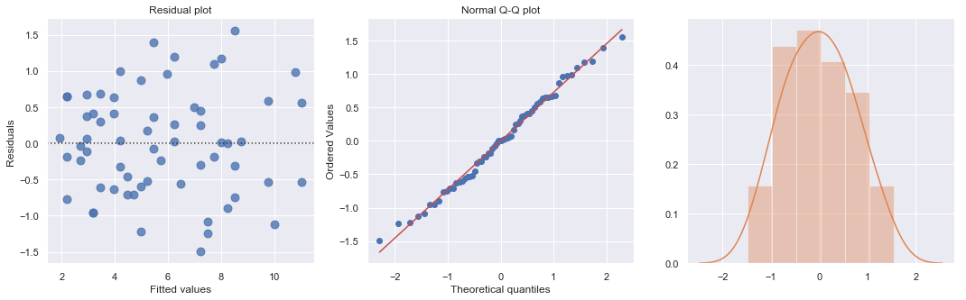
[18]:
df = pd.read_csv(dataurl+'costunits.csv', header=0, index_col='month')
df['units2'] = np.power(df.units,2)
result = ols(formula='cost ~ units + units2', data=df).fit()
display(result.summary())
fig, axes = plt.subplots(1,3,figsize=(18,6))
sns.residplot(result.fittedvalues, result.resid , lowess=False, scatter_kws={"s": 80},
              line_kws={'color':'r', 'lw':1}, ax=axes[0])
axes[0].set_title('Residual plot')
axes[0].set_xlabel('Fitted values')
axes[0].set_ylabel('Residuals')

axes[1].relim()
stats.probplot(result.resid, dist='norm', plot=axes[1])
axes[1].set_title('Normal Q-Q plot')
axes[2].relim()
sns.distplot(result.resid, ax=axes[2]);
plt.show()
toggle()
| Dep. Variable: | cost | R-squared: | 0.822 |
|---|---|---|---|
| Model: | OLS | Adj. R-squared: | 0.811 |
| Method: | Least Squares | F-statistic: | 75.98 |
| Date: | Mon, 20 May 2019 | Prob (F-statistic): | 4.45e-13 |
| Time: | 13:54:18 | Log-Likelihood: | -327.88 |
| No. Observations: | 36 | AIC: | 661.8 |
| Df Residuals: | 33 | BIC: | 666.5 |
| Df Model: | 2 | ||
| Covariance Type: | nonrobust |
| coef | std err | t | P>|t| | [0.025 | 0.975] | |
|---|---|---|---|---|---|---|
| Intercept | 5792.7983 | 4763.058 | 1.216 | 0.233 | -3897.717 | 1.55e+04 |
| units | 98.3504 | 17.237 | 5.706 | 0.000 | 63.282 | 133.419 |
| units2 | -0.0600 | 0.015 | -3.981 | 0.000 | -0.091 | -0.029 |
| Omnibus: | 2.245 | Durbin-Watson: | 2.123 |
|---|---|---|---|
| Prob(Omnibus): | 0.326 | Jarque-Bera (JB): | 2.021 |
| Skew: | -0.553 | Prob(JB): | 0.364 |
| Kurtosis: | 2.651 | Cond. No. | 5.12e+06 |
Warnings:
[1] Standard Errors assume that the covariance matrix of the errors is correctly specified.
[2] The condition number is large, 5.12e+06. This might indicate that there are
strong multicollinearity or other numerical problems.
[18]:
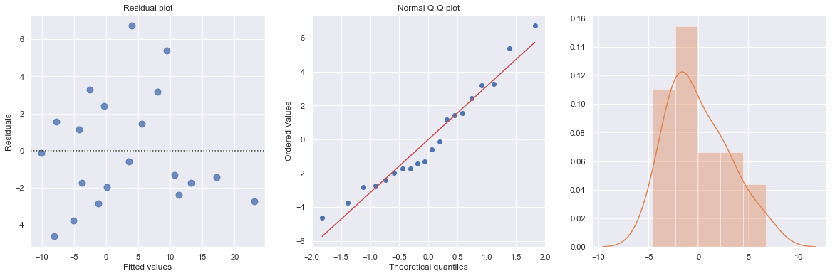
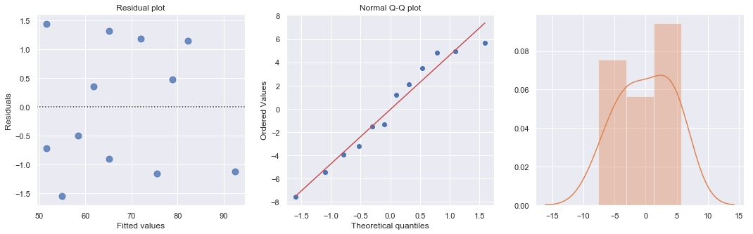
[19]:
df = pd.read_csv(dataurl+'carstopping.txt', delim_whitespace=True, header=0)
df['sqrtdist'] = np.sqrt(df.StopDist)
result = ols(formula='sqrtdist ~ Speed', data=df).fit()
fig, axes = plt.subplots(1,3,figsize=(18,5))
sns.residplot(result.fittedvalues, result.resid , lowess=False, scatter_kws={"s": 80},
              line_kws={'color':'r', 'lw':1}, ax=axes[0])
axes[0].set_title('Residual plot')
axes[0].set_xlabel('Fitted values')
axes[0].set_ylabel('Residuals')

axes[1].relim()
stats.probplot(result.resid, dist='norm', plot=axes[1])
axes[1].set_title('Normal Q-Q plot')
axes[2].relim()
sns.distplot(result.resid, ax=axes[2]);
plt.show()

toggle()
[19]:
Heteroscedasticity
Excessive nonconstant variance can create technical difficulties with a multiple linear regression model. For example, if the residual variance increases with the fitted values, then prediction intervals will tend to be wider than they should be at low fitted values and narrower than they should be at high fitted values. Some remedies for refining a model exhibiting excessive nonconstant variance includes the following:
Apply a variance-stabilizing transformation to the response variable, for example a logarithmic transformation (or a square root transformation if a logarithmic transformation is “too strong” or a reciprocal transformation if a logarithmic transformation is “too weak”).
Weight the variances so that they can be different for each set of predictor values. This leads to weighted least squares, in which the data observations are given different weights when estimating the model – see below.
A generalization of weighted least squares is to allow the regression errors to be correlated with one another in addition to having different variances. This leads to generalized least squares, in which various forms of nonconstant variance can be modeled.
For some applications we can explicitly model the variance as a function of the mean, E(Y). This approach uses the framework of generalized linear models.
[20]:
df = pd.read_csv(dataurl+'ca_learning.txt', sep='\s+', header=0)
result = analysis(df, 'cost', ['responses'], printlvl=4)
| Dep. Variable: | cost | R-squared: | 0.889 |
|---|---|---|---|
| Model: | OLS | Adj. R-squared: | 0.878 |
| Method: | Least Squares | F-statistic: | 80.19 |
| Date: | Mon, 20 May 2019 | Prob (F-statistic): | 4.33e-06 |
| Time: | 13:54:27 | Log-Likelihood: | -34.242 |
| No. Observations: | 12 | AIC: | 72.48 |
| Df Residuals: | 10 | BIC: | 73.45 |
| Df Model: | 1 | ||
| Covariance Type: | nonrobust |
| coef | std err | t | P>|t| | [0.025 | 0.975] | |
|---|---|---|---|---|---|---|
| Intercept | 19.4727 | 5.516 | 3.530 | 0.005 | 7.182 | 31.764 |
| responses | 3.2689 | 0.365 | 8.955 | 0.000 | 2.456 | 4.082 |
| Omnibus: | 2.739 | Durbin-Watson: | 1.783 |
|---|---|---|---|
| Prob(Omnibus): | 0.254 | Jarque-Bera (JB): | 1.001 |
| Skew: | 0.038 | Prob(JB): | 0.606 |
| Kurtosis: | 1.587 | Cond. No. | 63.1 |
Warnings:
[1] Standard Errors assume that the covariance matrix of the errors is correctly specified.
standard error of estimate:4.59830
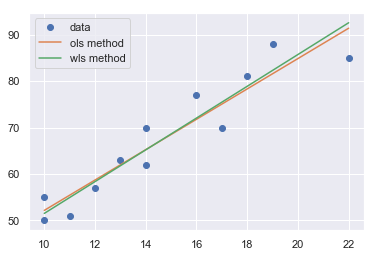
A plot of the residuals versus the predictor values indicates possible nonconstant variance since there is a very slight “megaphone” pattern. We therefore fit a simple linear regression model of the absolute residuals on the predictor and calculate weights as 1 over the squared fitted values from this model.
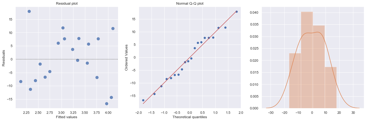
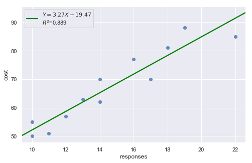
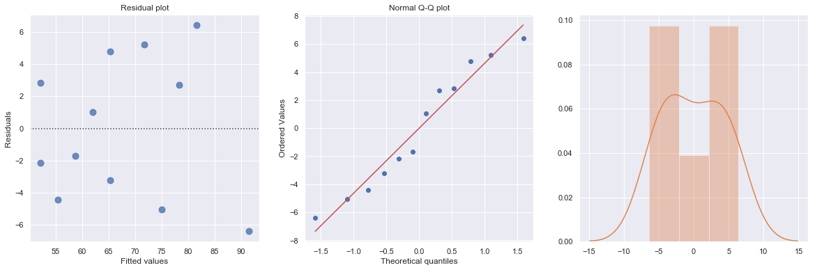
[21]:
result_ols = ols(formula='cost ~ responses', data=df).fit()
df['resid'] = abs(result_ols.resid)
result = ols(formula='resid ~ responses', data=df).fit()
X = sm.add_constant(df.responses)
w = 1./(result.fittedvalues ** 2)
result_wls = sm.WLS(df.cost, X, weights=w).fit()
display(result_wls.summary())
fig, axes = plt.subplots(1,3,figsize=(18,5))
sns.residplot(result_wls.fittedvalues, result_wls.wresid, lowess=False, scatter_kws={"s": 80},
              line_kws={'color':'r', 'lw':1}, ax=axes[0])
axes[0].set_title('Residual plot')
axes[0].set_xlabel('Fitted values')
axes[0].set_ylabel('Residuals')

axes[1].relim()
stats.probplot(result_wls.resid, dist='norm', plot=axes[1])
axes[1].set_title('Normal Q-Q plot')
axes[2].relim()
sns.distplot(result_wls.resid, ax=axes[2]);
plt.show()

x = np.linspace(np.min(df.responses), np.max(df.responses), 20)
y_wls = result_wls.params[0] + result_wls.params[1] * x
y_ols = result_ols.params[0] + result_ols.params[1] * x
plt.plot(df.responses, df.cost, 'o', label='data')
plt.plot(x, y_ols, '-', label='ols method')
plt.plot(x, y_wls, '-', label='wls method')
plt.legend()
plt.show()

toggle()
| Dep. Variable: | cost | R-squared: | 0.895 |
|---|---|---|---|
| Model: | WLS | Adj. R-squared: | 0.885 |
| Method: | Least Squares | F-statistic: | 85.35 |
| Date: | Mon, 20 May 2019 | Prob (F-statistic): | 3.27e-06 |
| Time: | 13:54:27 | Log-Likelihood: | -33.248 |
| No. Observations: | 12 | AIC: | 70.50 |
| Df Residuals: | 10 | BIC: | 71.47 |
| Df Model: | 1 | ||
| Covariance Type: | nonrobust |
| coef | std err | t | P>|t| | [0.025 | 0.975] | |
|---|---|---|---|---|---|---|
| const | 17.3006 | 4.828 | 3.584 | 0.005 | 6.544 | 28.058 |
| responses | 3.4211 | 0.370 | 9.238 | 0.000 | 2.596 | 4.246 |
| Omnibus: | 4.602 | Durbin-Watson: | 1.706 |
|---|---|---|---|
| Prob(Omnibus): | 0.100 | Jarque-Bera (JB): | 1.241 |
| Skew: | 0.062 | Prob(JB): | 0.538 |
| Kurtosis: | 1.429 | Cond. No. | 56.7 |
Warnings:
[1] Standard Errors assume that the covariance matrix of the errors is correctly specified.
[21]: