%run ../initscript.py
HTML("""
<div id="popup" style="padding-bottom:5px; display:none;">
    <div>Enter Password:</div>
    <input id="password" type="password"/>
    <button onclick="done()" style="border-radius: 12px;">Submit</button>
</div>
<button onclick="unlock()" style="border-radius: 12px;">Unclock</button>
<a href="#" onclick="code_toggle(this); return false;">show code</a>
""")

Enter Password:

Submit

Unclock show code

%run loadregfuncs.py
from ipywidgets import *
import warnings
warnings.filterwarnings('ignore')
%matplotlib inline
toggle()

show code

Regression Analysis

We consider a simple example to illustrate how to use python package statsmodels to perform regression analysis and predictions.

Influential Points

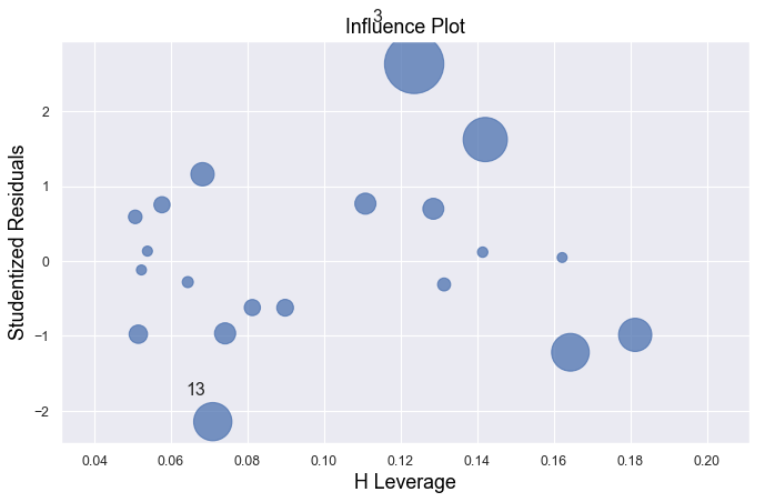
An influential point is an outlier that greatly affects the slope of the regression line. - An outlier is a data point whose response y does not follow the general trend of the rest of the data. - A data point has high leverage if it has “extreme” predictor x values. The lack of neighboring observations means that the fitted regression model will pass close to that particular observation.

Examples

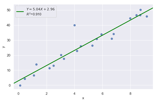
Example 1:

df = pd.read_csv(dataurl+'influence1.txt', delim_whitespace=True, header=0)
result = analysis(df, 'y', ['x'], printlvl=1)

fig, ax = plt.subplots(figsize=(10,6), dpi=80)
fig = sm.graphics.influence_plot(result, alpha  = 0.05, ax = ax, criterion="cooks")

Example 2:

df = pd.read_csv(dataurl+'influence2.txt', delim_whitespace=True, header=0)
result = analysis(df, 'y', ['x'], printlvl=1)

fig, ax = plt.subplots(figsize=(10,6), dpi=80)
fig = sm.graphics.influence_plot(result, alpha  = 0.05, ax = ax, criterion="cooks")

Example 3:

df = pd.read_csv(dataurl+'influence3.txt', delim_whitespace=True, header=0)
result = analysis(df, 'y', ['x'], printlvl=1)

fig, ax = plt.subplots(figsize=(10,6), dpi=80)
fig = sm.graphics.influence_plot(result, alpha  = 0.05, ax = ax, criterion="cooks")

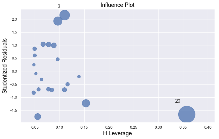
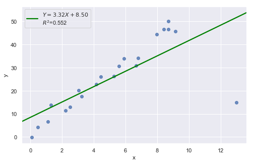
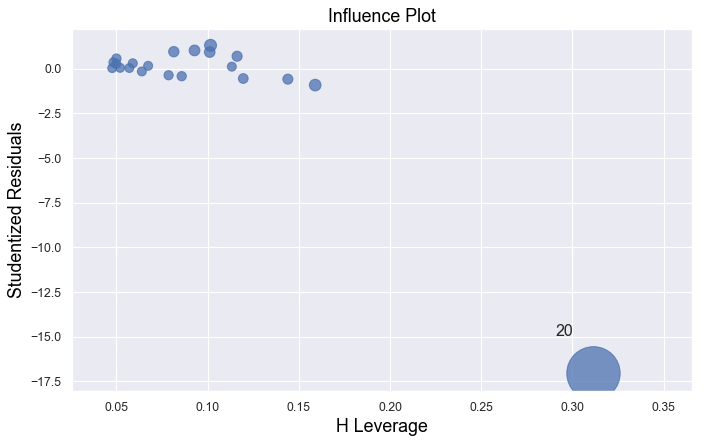
Example 4:

df = pd.read_csv(dataurl+'influence4.txt', delim_whitespace=True, header=0)
result = analysis(df, 'y', ['x'], printlvl=1)

fig, ax = plt.subplots(figsize=(10,6), dpi=80)
fig = sm.graphics.influence_plot(result, alpha  = 0.05, ax = ax, criterion="cooks")

In all examples above, do they contain outliers or high leverage data points? Are identified data points influential?

hide_answer()

show answer

If an observation has a studentized residual that is larger than 3 (in absolute value) we can call it an outlier.

Example 1:

All of the data points follow the general trend of the rest of the data, so there are no outliers (in the \(Y\) direction). And, none of the data points are extreme with respect to \(X\), so there are no high leverage points. Overall, none of the data points would appear to be influential with respect to the location of the best fitting line.

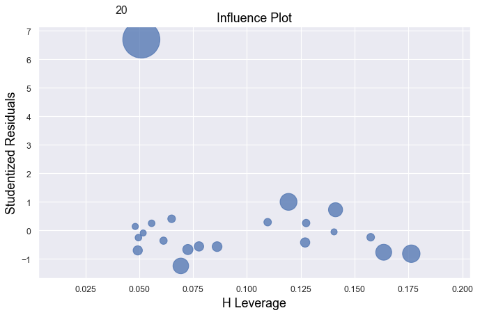
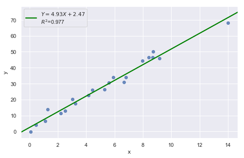
Example 2:

There is one outlier, but no high leverage points. An easy way to determine if the data point is influential is to find the best fitting line twice — once with the red data point included and once with the red data point excluded. The data point is not influential.

Example 3:

The data point is not influential, nor is it an outlier, but it does have high leverage.

Example 4:

The data point is deemed both high leverage and an outlier, and it turned out to be influential too.

Partial Regression Plots

For a particular independent variable \(X_i\), a partial regression plot shows:

• residuals from regressing \(Y\) (the response variable) against all the independent variables except \(X_i\)

• residuals from regressing \(X_i\) against the remaining independent variables.

It has a slope that is the same as the multiple regression coefficient for that predictor and also has the same residuals as the full multiple regression. So we can spot any outliers or influential points and tell whether they’ve affected the estimation of this particular coefficient. For the same reasons that we always look at a scatterplot before interpreting a simple regression coefficient, it’s a good idea to make a partial regression plot for any multiple regression coefficient that we hope to understand or interpret.

ANOVA

ANOVA Table

Consider the heart attacks in rabbits study with variables: - the infarcted area (in grams) of a rabbit - the region at risk (in grams) of a rabbit - x2=1 if early cooling of a rabbit, 0 if not - x3=1 if late cooling of a rabbit, 0 if not

The regress formula is

\begin{equation*} \text{Infarc} = \beta_0 + \beta_1 \times \text{Area} + \beta_2 \times \text{X2} + \beta_3 \times \text{X3} \end{equation*}

df = pd.read_csv(dataurl+'coolhearts.txt', delim_whitespace=True, header=0)
result = analysis(df, 'Infarc', ['Area','X2','X3'], printlvl=0)
sm.stats.anova_lm(result, typ=2)

	sum_sq	df	F	PR(>F)
Area	0.637420	1.0	32.753601	0.000004
X2	0.297327	1.0	15.278050	0.000536
X3	0.019814	1.0	1.018138	0.321602
Residual	0.544910	28.0	NaN	NaN

• sum_sq[Residual] is sum of squared residuals;

• sum_sq[Area] is sum_sq[Residual] - sum_sq[Residual] for regression Infarc ~ X2 + X3, i.e., regression without Area;

• df[Residual] is degree of freedom \(=\) total number of observations (result.nobs) \(-\) the number of explanatory variables (3 or result.df_model) \(- 1 =\) result.df_resid;

Examples

ANOVA (analysis of variance) table for regression can be used to test hypothesis:

\begin{align} H_0:& \text{ a subset of explanatory variables have $0$ slope} \nonumber\\ H_a:& \text{ at least one variable in the subset of explanatory variables have nonzero slope} \nonumber \end{align}

Example 1: \begin{align} H_0:& \quad \beta_i = 0 ~ \forall i \in \{1\} \nonumber\\ H_a:& \quad \beta_i \neq 0 \text{ for at least one } i \in \{1\}. \nonumber \end{align}

df = pd.read_csv(dataurl+'coolhearts.txt', delim_whitespace=True, header=0)
_ = GL_Ftest(df, 'Infarc', ['Area','X2','X3'], ['X2','X3'], 0.05)

The F-value is 32.754 and p-value is 0.000. Reject null hypothesis.
At least one variable in {'Area'} has nonzero slope.

It shows the size of the infarct is significantly related to the size of the area at risk. The result of such F-test is always equivalent to the t-test result.

Example 2: \begin{align} H_0:& \quad \beta_i = 0 ~ \forall i \in \{1,2,3\} \nonumber\\ H_a:& \quad \beta_i \neq 0 \text{ for at least one } i \in \{1,2,3\}. \nonumber \end{align}

df = pd.read_csv(dataurl+'coolhearts.txt', delim_whitespace=True, header=0)
_ = GL_Ftest(df, 'Infarc', ['Area','X2','X3'], [], 0.05)

The F-value is 16.431 and p-value is 0.000. Reject null hypothesis.
At least one variable in {'Area', 'X2', 'X3'} has nonzero slope.

This is also called a test for the overall fit. The F-statistics and its p value are also available from the fvalue and f_pvalue properties of the regression result in statsmodels.

Example 3: \begin{align} H_0:& \quad \beta_i = 0 ~ \forall i \in \{2,3\} \nonumber\\ H_a:& \quad \beta_i \neq 0 \text{ for at least one } i \in \{2,3\}. \nonumber \end{align}

df = pd.read_csv(dataurl+'coolhearts.txt', delim_whitespace=True, header=0)
_ = GL_Ftest(df, 'Infarc', ['Area','X2','X3'], ['Area'], 0.05)

The F-value is 8.590 and p-value is 0.001. Reject null hypothesis.
At least one variable in {'X2', 'X3'} has nonzero slope.

Summary

Let \(K \subseteq N\), we have two hypothesis \begin{align} H_0:& \quad \beta_i = 0 ~ \forall i \in K \nonumber\\ H_a:& \quad \beta_i \neq 0 \text{ for at least one } i \in K. \nonumber \end{align}

We consider two models \begin{align} \text{full model:} & \quad Y = \beta_0 + \sum_{i \in N} \beta_i X_i \nonumber\\ \text{reduced model:} & \quad Y = \beta_0 + \sum_{i \in K} \beta_i X_i. \nonumber\\ \end{align}

Let \(SSE(F)\) and \(SSE(R)\) be the sum of squared errors for the full and reduced models respectively where

\begin{equation*} SSE = \text{sum of squared residuals} = \sum e^2_i = \sum (Y_i - \hat{Y}_i)^2. \end{equation*}

The general linear statistic:

\begin{equation*} F^\ast = \frac{SSE(R) - SSE(F)}{df_R - df_F} \div \frac{SSE(F)}{df_F} \end{equation*}

and \(p\)-value is \begin{equation*} 1 - \text{F-dist}(F^\ast, df_R - df_F, df_F). \end{equation*}

Why don’t we perform a series of individual t-tests? For example, for the rabbit heart attacks study, we could have done the following in Example 3:

• Fit the model InfSize ~ Area \(+\) x2 \(+\) x3 and use an individual t-test for x3.

• If the test results indicate that we can drop x3 then fit the model oInfSize ~ Area \(+\) x2 and use an individual t-test for x2.

hide_answer()

show answer

Note that we’re using two individual t-tests instead of one F-test in the suggested method. It means the chance of drawing an incorrect conclusion in our testing procedure is higher. Recall that every time we do a hypothesis test, we can draw an incorrect conclusion by:

• rejecting a true null hypothesis, i.e., make a type 1 error by concluding the tested predictor(s) should be retained in the model, when in truth it/they should be dropped; or

• failing to reject a false null hypothesis, i.e., make a type 2 error by concluding the tested predictor(s) should be dropped from the model, when in truth it/they should be retained.

Thus, in general, the fewer tests we perform the better. In this case, this means that wherever possible using one F-test in place of multiple individual t-tests is preferable.

Prediction

After we have estimated a regression equation from a dataset, we can use this equation to predict the value of the dependent variable for new observations.

df = pd.read_csv(dataurl+'costs.csv', header=0, index_col='month')
result = analysis(df, 'cost', ['production_runs','machine_hours'], printlvl=0)

df_pred = pd.DataFrame({'machine_hours':[1430, 1560, 1520],'production_runs': [35,45,40]})
predict = result.get_prediction(df_pred)
predict.summary_frame(alpha=0.05)

	mean	mean_se	mean_ci_lower	mean_ci_upper	obs_ci_lower	obs_ci_upper
0	97180.354898	697.961311	95760.341932	98600.367863	88700.800172	105659.909623
1	111676.265905	1135.822591	109365.417468	113987.114342	103002.948661	120349.583149
2	105516.720354	817.257185	103853.998110	107179.442598	96993.161428	114040.279281

• mean is the value calculated based on the (sample) regression line

• mean (or confidence) lower and upper limits offer the confidence interval of the average of predictor with given values of explanatory variables. In other words, if we run experiments many times with given values of explanatory variables, we have 95% confidence that the mean of the dependent variable will be in this interval.

• obs (or prediction) lower and upper limits offer the confidence interval of a single prediction. In other words, if we run one experiment with given values of explanatory variables, we have 95% confidence that the value of the dependent variable will be in this interval.

Cross Validation

The fit from a regression analysis is often overly optimistic (over-fitted). There is no guarantee that the fit will be as good when th estimated regression equation is applied to new data.

To validate the fit, we can gather new data, predict the dependent variable and compare with known values of the dependent variable. However, most of the time we cannot obtain new independent data to validate our model. An alternative is to partition the sample data into a training set and testing (validation) set.

The simplest approach to cross-validation is to partition the sample observations randomly with 50% of the sample in each set or 60%/40% or 70%/30%.

df = pd.read_csv(dataurl+'costs.csv', header=0, index_col='month')
result = analysis(df, 'cost', ['production_runs','machine_hours'], printlvl=0)

df_validate = pd.read_csv(dataurl+'validation.csv', header=0)
predict = result.get_prediction(df_validate)
df_validate['predict'] = predict.predicted_mean
r2 = np.corrcoef(df_validate.cost,df_validate.predict)[0,1]**2
stderr = np.sqrt(((df_validate.cost - df_validate.predict)**2).sum()/df_validate.shape[0]-3)
print('Validation R-squared:\t\t{:.3f}'.format(r2))
print('Validation StErr of Est:\t{:.3f}'.format(stderr))

Validation R-squared:           0.773
Validation StErr of Est:        5032.718

\(K\)-fold cross-validation can also be used. This partitions the sample dataset into \(K\) subsets with equal size. For each subset, we use it as testing set and the remaining \(K-1\) subsets as training set. We then calculate the sum of squared prediction errors, and combine the \(K\) estimates of prediction error to produce a \(K\)-fold cross-validation estimate.

Multicollinearity

Multicollinearity exists when two or more of the predictors in a regression model are moderately or highly correlated with one another. The exact linear relationship is fairly simple to spot because regression packages will typically respond with an error message. A more common and serious problem is multicollinearity, where explanatory variables are highly, but not exactly, correlated.

There are two types of multicollinearity:

• Structural multicollinearity is a mathematical artifact caused by creating new predictors from other predictors — such as, creating the predictor \(X^2\) from the predictor \(X\).

• Data-based multicollinearity, on the other hand, is a result of a poorly designed experiment, reliance on purely observational data, or the inability to manipulate the system on which the data are collected.

Variance inflation factor (VIF) can be used to identify multicollinearity. The VIF for \(X\) is defined as 1/(1 - R-square for \(X\)), where R-square for \(X\) variable is the usual R-square value from a regression with that \(X\) as the dependent variable and the other \(X\)’s as the explanatory variables.

from statsmodels.stats.outliers_influence import variance_inflation_factor
from patsy import dmatrices

df = pd.read_csv(dataurl+'multicollinearity.csv',header=0, index_col='person')
features = "+".join(df.drop(columns=['salary']).columns)
y, X = dmatrices('salary ~' + features, df, return_type='dataframe')
VIF = pd.DataFrame()
VIF["VIF Factor"] = [variance_inflation_factor(X.values, i) for i in range(1,X.shape[1])]
VIF["Features"] = X.drop(columns=['Intercept']).columns
display(VIF)

def calculate_vif_(X, thresh=5.0):
    cols = X.columns
    variables = np.arange(X.shape[1])
    dropped=True
    while dropped:
        dropped=False
        c = X[cols[variables]].values
        vif = [variance_inflation_factor(c, ix) for ix in np.arange(c.shape[1])]

        maxloc = vif.index(max(vif))
        if max(vif) > thresh:
            print('dropping \'' + X[cols[variables]].columns[maxloc] + '\' at index: ' + str(maxloc))
            variables = np.delete(variables, maxloc)
            dropped=True

    print('Remaining variables:')
    print(X.columns[variables])

calculate_vif_(X.drop(columns=['Intercept']))
toggle()

	VIF Factor	Features
0	1.001383	gender[T.Male]
1	31.503655	age
2	38.153090	experience
3	5.594549	seniority

dropping 'experience' at index: 2
dropping 'age' at index: 1
Remaining variables:
Index(['gender[T.Male]', 'seniority'], dtype='object')

show code