%run ../initscript.py
HTML("""
<div id="popup" style="padding-bottom:5px; display:none;">
    <div>Enter Password:</div>
    <input id="password" type="password"/>
    <button onclick="done()" style="border-radius: 12px;">Submit</button>
</div>
<button onclick="unlock()" style="border-radius: 12px;">Unclock</button>
<a href="#" onclick="code_toggle(this); return false;">show code</a>
""")

Enter Password:

Submit

Unclock show code

%run ./loadoptfuncs.py
toggle()

show code

Nonlinear Programming

In many optimization models the objective and/or the constraints are nonlinear functions of the decision variables. Such an optimization model is called a nonlinear programming (NLP) model.

• When you solve an LP model, you are mostly guaranteed that the solution obtained is an optimal solution and a sensitivity analysis with shadow price and reduced cost is available.

• When you solve an NLP model, it is very possible that you obtain a suboptimal solution.

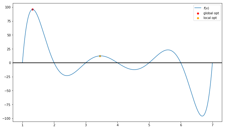
This is because a nonlinear function can have local optimal solutions where

• a local optimum is better than all nearby points

that are not the global optimal solution

• a global optimum is the best point in the entire feasible region

draw_local_global_opt()

However, convex programming, as one of the most important type of nonlinear programming models, can be solved to its optimality.

interact(showconvex,
         values = widgets.FloatRangeSlider(value=[2, 3.5],
                                           min=1.0, max=4.0, step=0.1,
                                           description='Test:', disabled=False,
                                           continuous_update=False,
                                           orientation='horizontal',readout=True,
                                           readout_format='.1f'));

Gradient Decent Algorithm

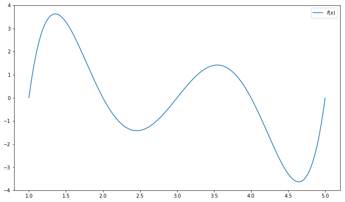
The gradient decent algorithm performs as the core part of many general purpose algorithms for solving NLP models. Consider a function

\begin{equation*} f(x) = (x-1) \times (x-2) \times (x-3) \times (x-4) \times (x-5) \end{equation*}

function = lambda x: (x-1)*(x-2)*(x-3)*(x-4)*(x-5)
x = np.linspace(1,5,500)
plt.figure(figsize=(12,7))
plt.plot(x, function(x), label='$f(x)$')
plt.legend()
plt.show()

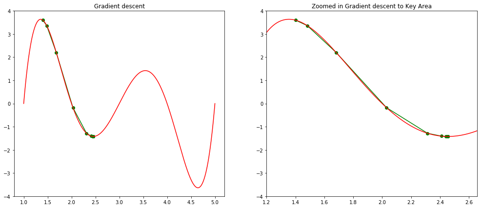
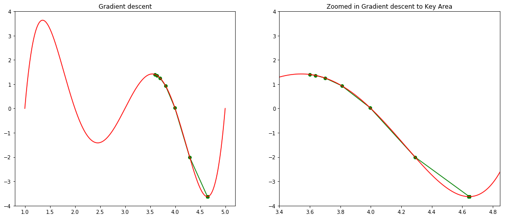
The gradient decent algorithm is typically used to find a local minimum with given initial solution. In our visual demonstration, a global optimal is found by using 3.6 as initial solution.

As it is usually impossible to identify the best initial solution, multistart option is often used in NLP solver, which will randomly select a large amount of initial solutions and run solver parallely.

step(1.4, 0, 0.001, 0.05)
step(3.6, 0, 0.001, 0.05)

Local minimum occurs at: 2.4558826297046497
Number of steps: 11

Local minimum occurs at: 4.644924463813627
Number of steps: 67

Genetic Algorithms

In the early 1970s, John Holland of the University of Michigan realized that many features espoused in the theory of natural evolution, such as survival of the fittest and mutation, could be used to help solve difficult optimization problems. Because his methods were based on behavior observed in nature, Holland coined the term genetic algorithm to describe his algorithm. Simply stated, a genetic algorithm (GA) provides a method of intelligently searching an optimization model’s feasible region for an optimal solution.

The process of natural selection starts with the selection of fittest individuals from a population. They produce offspring which inherit the characteristics of the parents and will be added to the next generation. If parents have better fitness, their offspring will be better than parents and have a better chance at surviving. This process keeps on iterating and at the end, a generation with the fittest individuals will be found.

population = {
    'A1': '000000',
    'A2': '111111',
    'A3': '101011',
    'A4': '110110'
}
population

{'A1': '000000', 'A2': '111111', 'A3': '101011', 'A4': '110110'}

Biological terminology is used to describe the algorithm: - The objective function is called a fitness function. - An individual is characterized by a set of parameters known as Genes. Genes are joined into a string to form a Chromosome (variable or solution). - The set of genes of an individual is represented by using a string of binary values (i.e., string of \(1\)s and \(0\)s). We say that we encode the genes in a chromosome. For example, - 1001 in binary system represents \(1 \times (2^3) + 0 \times (2^2) + 0 \times (2^1) + 1 \times (2^0) = 8 + 1 = 9\) in decimal system - It is similar to how 1001 is represented in decimal system \(1 \times (10^3) + 0\times (10^2) + 0 \times (10^1) + 1 \times (10^0) = 1000 + 1 = 1001\)

{key:int(value,2) for key,value in population.items()}

{'A1': 0, 'A2': 63, 'A3': 43, 'A4': 54}

GA uses the following steps: 1. Generate a population. The GA randomly samples values of the changing cells between the lower and upper bounds to generate a set of (usually at least 50) chromosomes. The initial set of chromosomes is called the population.

2. Create a new generation. Create a new generation of chromosomes in the hope of finding an improvement. In the new generation, chromosomes with a larger fitness function (in a maximization problem) have a greater chance of surviving to the next generation.

   • Crossover and mutation are also used to generate chromosomes for the next generation.

   • Crossover (fairly common) splices together two chromosomes at a pre-specified point.

   • Mutation (very rare) randomly selects a digit and changes it from 0 to 1 or vice versa.

   For example, consider the crossover point to be 3 as shown below.

   Offspring are created by exchanging the genes of parents among themselves until the crossover point is reached.

   The new offspring A5 and A6 are added to the population.

   
   

   A5 may mutate

3. Stopping condition. At each generation, the best value of the fitness function in the generation is recorded, and the algorithm repeats step 2. If no improvement in the best fitness value is observed after many consecutive generations, the GA terminates.

Strengths of GA: - If you let a GA run long enough, it is guaranteed to find the solution to any optimization problem. - GAs do very well in problems with few constraints. The complexity of the objective cell does not bother a GA. For example, a GA can easily handle MIN, MAX, IF, and ABS functions in the models. This is the key advantage of GAs.

Weakness of GA: - It might take too long to find a good solution. Even a solution is found, you do not know if the solution is optimal or how close it is to the optimal solution. - GAs do not usually perform very well on problems that have many constraints. For example, Simplex LP Solver has no difficulty with the multiple-constraint linear models, but GAs perform much worse and more slowly on them.

Application: Traveling salesman problem (TSP)

The TSP has several applications even in its purest formulation, such as planning, logistics, and the manufacture of microchips. TSP is a touchstone for many general heuristics devised for combinatorial optimization such as genetic algorithms.

HTML('<iframe width="560" height="315" src="https://www.youtube-nocookie.com/embed/CsJRsToDI8w" frameborder="0" allow="accelerometer; autoplay; encrypted-media; gyroscope; picture-in-picture" allowfullscreen></iframe>')

Summary

Consider an optimization problem

\begin{align*} \min & \quad f(x) \\ \text{subject to} & \quad h_i(x) \geq 0 \quad \forall i = 1, \ldots, n \end{align*}

If the objective function and constraints are all convex functions, then it is a convex problem, otherwise it is a non-convex problem.

In general, commercial software, such as CPLEX or Gurobi,

• can find an optimal solution for convex problem, for example, linear programming.

• use branch-and-bound algorithm to solve mixed-integer programming, which is generally a non-convex problem. Although it cannot guarantee a global optimal solution, it can provide an optimality gap to show the solution quality.

• can only find a local optimal for general non-convex problem without knowing solution quality.