[1]:
%run ../initscript.py
HTML("""
<div id="popup" style="padding-bottom:5px; display:none;">
    <div>Enter Password:</div>
    <input id="password" type="password"/>
    <button onclick="done()" style="border-radius: 12px;">Submit</button>
</div>
<button onclick="unlock()" style="border-radius: 12px;">Unclock</button>
<a href="#" onclick="code_toggle(this); return false;">show code</a>
""")
[1]:
[2]:
# import pandas as pd
# import numpy as np
# import matplotlib.pyplot as plt
# from matplotlib.path import Path
# from matplotlib.patches import PathPatch
# import seaborn as sns
# # from pulp import *

# from ipywidgets import *
# %matplotlib inline
# import warnings
# warnings.filterwarnings('ignore')
%run ./loadoptfuncs.py
toggle()
[2]:
Mixed-Integer Programming
Optimization models in which some or all of the variables must be integer are known as mixed-integer programming (MIP). There are two main reasons for using MIP.
The decision variables are quantities that have to be integer, e.g., number of employee to assign or number of car to make
The decision variables are binaries to indicate whether an activity is undertaken, e.g., \(z=0\) or \(1\) where \(1\) indicates the decision of renting an equipment so that the firm need to pay a fixed cost, \(0\) otherwise.
If we relax the integrality requirements of MIP, then we obtain a so-called LP relaxation of a given MIP.
You might suspect that MIP would be easier to solve than LP models. After all, there are only a finite number of feasible integer solutions in an MIP model, whereas there are infinitely many feasible solutions in an LP model.
However, exactly the opposite is true. MIP models are considerably harder than LP models, because the optimal solution rarely occurs at the corner of its LP relaxation. Algorithms such as Branch-and-bound (B&B) or Branch-and-cut (B&C) are designed for solving MIP effectively and well implemented in commercial software.
Branch and Bound Algorithm
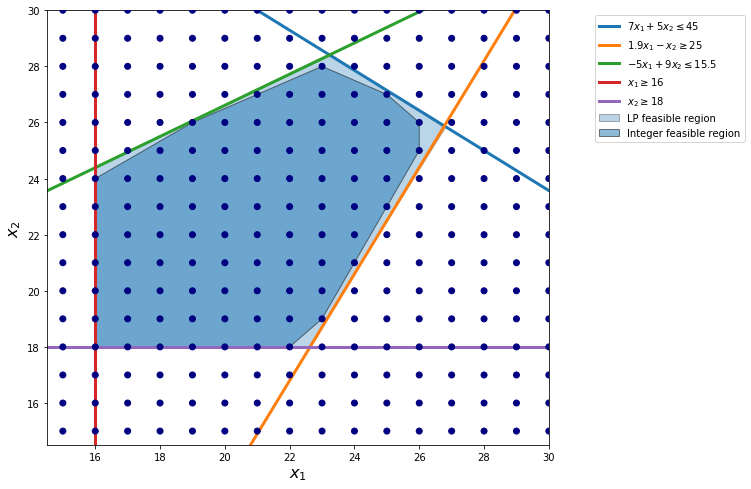
Branch-and-bound algorithm is designed to use LP relaxation to solve MIP. The picture shows the difference between a MIP and its LP relaxation.
The “integer feasible region” in the picture connects all integer feasible solutions. In particular, it is a convex combination of all feasible solutions.
Similar to LP, the optimal solution of the MIP occurs at the corner of the integer feasible region.
However, as shown in the picture, the boundary of integer feasible region is much more complicated than its LP relaxation feasible region.
[3]:
show_integer_feasregion()
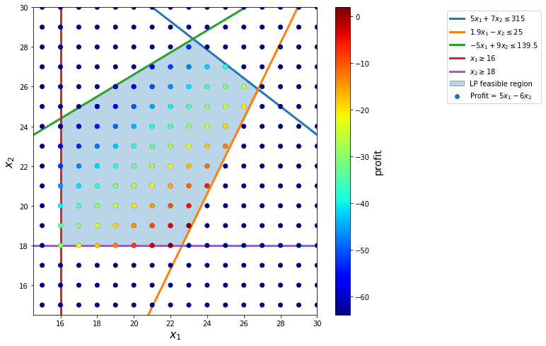
We demonstrate branch-and-bound procedure as follows.
[4]:
from ipywidgets import widgets
from IPython.display import display, Math
from traitlets import traitlets
class LoadedButton(widgets.Button):
"""A button that can holds a value as a attribute."""
def __init__(self, value=None, *args, **kwargs):
super(LoadedButton, self).__init__(*args, **kwargs)
# Create the value attribute.
self.add_traits(value=traitlets.Any(value))
def add_num(ex):
ex.value = ex.value+1
if ex.value<=3:
fig, ax = plt.subplots(figsize=(9, 8))
ax.set_xlim(15-0.5, 30)
ax.set_ylim(15-0.5, 30)
s = np.linspace(0, 50)
plt.plot(s, 45 - 5*s/7, lw=3, label='$5x_1 + 7x_2 \leq 315$')
plt.plot(s, -25 + 1.9*s, lw=3, label='$1.9x_1 - x_2 \leq 25$')
plt.plot(s, 15.5 + 5*s/9, lw=3, label='$-5x_1 + 9x_2 \leq 139.5$')
plt.plot(16 * np.ones_like(s), s, lw=3, label='$x_1 \geq 16$')
plt.plot(s, 18 * np.ones_like(s), lw=3, label='$x_2 \geq 18$')
# plot the possible (x1, x2) pairs
pairs = [(x1, x2) for x1 in np.arange(start=15, stop=31, step=1)
for x2 in np.arange(start=15, stop=31, step=1)]
# split these into our variables
x1, x2 = np.hsplit(np.array(pairs), 2)
# plot the results
plt.scatter(x1, x2, c=0*x1 - 0*x2, cmap='jet', zorder=3)
feaspairs = [(x1, x2) for x1 in np.arange(start=15, stop=31, step=1)
for x2 in np.arange(start=15, stop=31, step=1)
if (5/7*x1 + x2) <= 45
and (-1.9*x1 + x2) >= -25
and (-5/9*x1 + x2) <= 15.5
and x1>=16 and x2>=18]
# split these into our variables
x1, x2 = np.hsplit(np.array(feaspairs), 2)
# plot the results
plt.scatter(x1, x2, c=5*x1 - 6*x2, label='Profit = $5x_1 - 6x_2$', cmap='jet', zorder=3)
if ex.value>=3:
bpath1 = Path([
(16., 18.),
(16., 24.4),
(22, 27.8),
(22, 27),
(22, 18.),
(16., 18.),
])
bpatch1 = PathPatch(bpath1, label='New feasible region', alpha=0.5)
ax.add_patch(bpatch1)
bpath2 = Path([
(23., 18.7),
(23., 28.2),
(23.2,28.4),
(26.8, 25.8),
(23., 18.7),
])
bpatch2 = PathPatch(bpath2, label='New feasible region', alpha=0.5)
ax.add_patch(bpatch2)
cb = plt.colorbar()
cb.set_label('profit', fontsize=14)
plt.xlim(15-0.5, 30)
plt.ylim(15-0.5, 30)
plt.xlabel('$x_1$', fontsize=16)
plt.ylabel('$x_2$', fontsize=16)
lppath = Path([
(16., 18.),
(16., 24.4),
(23.3, 28.4),
(26.8, 25.8),
(22.6, 18.),
(16., 18.),
])
lppatch = PathPatch(lppath, label='LP feasible region', alpha=0.3)
ax.add_patch(lppatch)
if ex.value==1:
display(Math('Show~feasible~region...'))
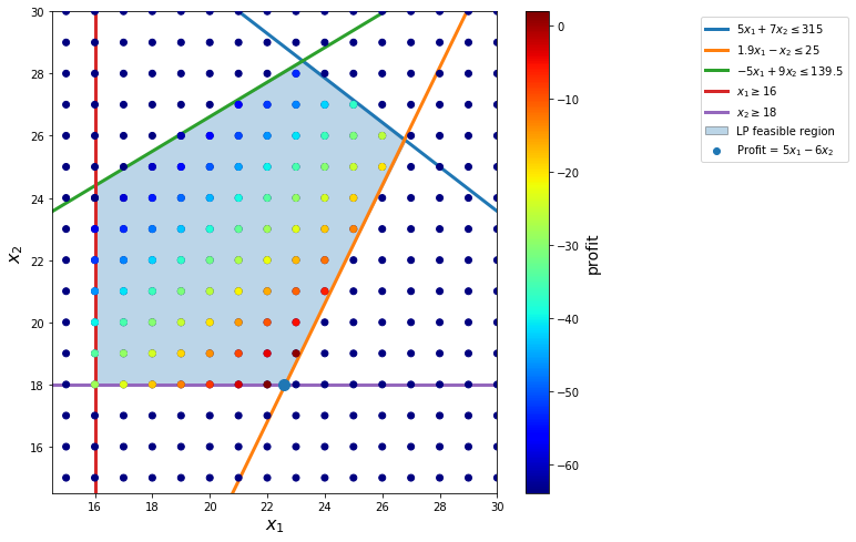
if ex.value==2:
display(Math('Solve~linear~programming...'))
display(Math('\nThe~solution~is~x_1 = {:.3f}, x_2={}~with~profit={}'.format(22.632,18,5.158)))
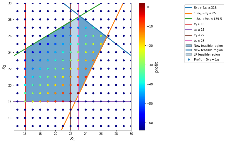
if ex.value==3:
display(Math('The~solution~is~integer~infeasible.~So~we~use~branch~and~bound.'))
display(Math('Branch~LP~feasible~region~into~two:~x_1 \le 22~and~x_1 \ge 23,~and~solve~two~LPs.'))
display(Math('Bound~the~optimal~profit~from~above~with~5.158.'))
if ex.value==2:
plt.scatter([22.57], [18], s=[100], zorder=4)
if ex.value>=3:
plt.plot(22 * np.ones_like(s), s, lw=3, label='$x_1 \leq 22$')
plt.plot(23 * np.ones_like(s), s, lw=3, label='$x_1 \geq 23$')
plt.legend(fontsize=18)
ax.legend(loc='upper right', bbox_to_anchor=(1.8, 1))
plt.show()
# lb = LoadedButton(description="Next", value=0)
# lb.on_click(add_num)
# display(lb)
class ex:
value = 1
for i in range(3):
ex.value = i
add_num(ex)
toggle()
[4]:
The Branch-and-bound algorithm keeps a tree structure in its solving process.
Modeling with Binary Variables
A binary variable usually corresponds to an activity that is or is not undertaken. We can model logics by using constraints involving binary variables.
For example, let \(z_1, \ldots, z_5\) be variables to indicate whether we will order products from suppliers \(1, \ldots, 5\) respectively.
The logic “if you use supplier 2, you must also use supplier 1” can be modeled as
\begin{align} z_2 \le z_1 \nonumber \end{align}
The logic “if you use supplier 4, you may NOT use supplier 5” can be modeled as
\begin{align} z_4 + z_5 \le 1 \nonumber \end{align}
Example: Facility Location
Consider the classic facility location problem. Given
a set \(L\) of customer locations and
a set \(F\) of candidate facility sites
We must decide on which sites to build facilities and assign coverage of customer demand to these sites so as to minimize cost.
All customer demand \(d_ i\) must be satisfied, and each facility has a demand capacity limit \(C\).
The total cost is the sum of the distances \(c_{ij}\) between facility \(j\) and its assigned customer \(i\), plus a fixed charge \(f_ j\) for building a facility at site \(j\).
Let \(y_ j = 1\) represent choosing site \(j\) to build a facility, and 0 otherwise. Also,
let \(x_{ij} = 1\) represent the assignment of customer \(i\) to facility \(j\), and 0 otherwise.
This model can be formulated as the following integer linear program:
Constraint (2) ensures that each customer is assigned to exactly one site.
Constraint (3) forces a facility to be built if any customer has been assigned to that facility.
Finally, constraint (4) enforces the capacity limit at each site.
\begin{align} \min & \quad \sum_{i \in L} \sum_{j \in F} c_{ij} x_{ij} + \sum_{j \in F} f_j y_j \\ \text{s.t.} & \quad \sum_{j \in F} x_{ij} = 1 && \forall i \in L \\ & \quad x_{ij} \leq y_j && \forall i \in L, j \in F \\ & \quad \sum_{i \in L} d_i x_{ij} \le C y_j && \forall j \in F \\ & \quad x_{ij} \in \{0,1\}, y_j \in \{0,1\} && \forall i \in L, j \in F \end{align}
SAS Log for MIP
NOTE: The Branch and Cut algorithm is using up to 2 threads.
          Node   Active   Sols    BestInteger      BestBound      Gap    Time
             0        1      5  13138.9827130              0    13139       0
             0        1      5  13138.9827130   9946.2514269   32.10%       0
             0        1      5  13138.9827130   9964.0867656   31.86%       0
             0        1      5  13138.9827130   9972.4224200   31.75%       0
             0        1      7  11165.8124056   9975.2866538   11.93%       0
             0        1      7  11165.8124056   9977.8057106   11.91%       0
             0        1      7  11165.8124056   9978.9372347   11.89%       0
             0        1      7  11165.8124056   9980.8568737   11.87%       0
             0        1      9  10974.7644641   9982.4953533    9.94%       0
NOTE: The MILP solver added 17 cuts with 492 cut coefficients at the root.
           100       37     10  10961.8123535  10380.2158229    5.60%       0
           121       44     11  10954.3760034  10938.0514190    0.15%       0
           131       48     12  10951.0805543  10941.1165997    0.09%       0
           139       49     13  10948.4603465  10941.1165997    0.07%       0
           187        8     13  10948.4603465  10947.3813808    0.01%       0
NOTE: Optimal within relative gap.
NOTE: Objective = 10948.460347.
Although a MIP problem sometimes can be difficult to solve to its optimality, the gap column provides us useful information on solution quality. It shows that the objective value of the best integer solution the solver find so far is within a certain percentage gap of the true underlying optimal solution.