%run loadmlfuncs.py

Naive Bayes

Naive Bayes models are a group of extremely fast and simple classification algorithms that are often suitable for very high-dimensional datasets. Because they are so fast and have so few tunable parameters, they end up being very useful as a quick-and-dirty baseline for a classification problem. This section will focus on an intuitive explanation of how naive Bayes classifiers work.

Bayesian Classification

Naive Bayes classifiers are built on Bayesian classification methods. These rely on Bayes’s theorem, which is an equation describing the relationship of conditional probabilities of statistical quantities.

In Bayesian classification, we’re interested in finding the probability of a label given some observed features, which we can write as \(P(C~|~{\rm features})\). Bayes’s theorem tells us how to express this in terms of quantities we can compute more directly:

\[P(C~|~{\rm features}) = \frac{P({\rm features}~|~C)P(C)}{P({\rm features})}\]

If we are trying to decide between two labels — let’s call them \(C_1\) and \(C_2\) — then one way to make this decision is to compute the ratio of the posterior probabilities for each label:

\[\frac{P(C_1~|~{\rm features})}{P(C_2~|~{\rm features})} = \frac{P({\rm features}~|~C_1)}{P({\rm features}~|~C_2)}\frac{P(C_1)}{P(C_2)}\]

All we need now is some model by which we can compute \(P({\rm features}~|~C_i)\) for each label. Such a model is called a generative model because it specifies the hypothetical random process that generates the data.

Specifying this generative model for each label is the main piece of the training of such a Bayesian classifier. The general version of such a training step is a very difficult task, but we can make it simpler through the use of some simplifying assumptions about the form of this model.

This is where the “naive” in “naive Bayes” comes in: if we make very naive assumptions about the generative model for each label, we can find a rough approximation of the generative model for each class, and then proceed with the Bayesian classification.

Bernoulli Naive Bayes

There are 856 people who have either tried or not tried a company’s new frozen lasagna product. The data includes the categorical dependent variable tried and several other explanatory variables.

df_lasagna = pd.read_csv(dataurl+'lasagna.csv', header=0, index_col='person')
df_lasagna.head()

	age	weight	income	car_value	debt	mall_trips	gender	alone	dwell	pay_type	nbhd	tried
person
1	48	175	65500	2190	3510	7	Male	No	Home	Hourly	East	No
2	33	202	29100	2110	740	4	Female	No	Condo	Hourly	East	Yes
3	51	188	32200	5140	910	1	Male	No	Condo	Salaried	East	No
4	56	244	19000	700	1620	3	Female	No	Home	Hourly	West	No
5	28	218	81400	26620	600	3	Male	No	Apt	Salaried	West	Yes

For the Naive Bayes method, numeric predictors must be binned, i.e., made categorical. For this example, each numeric variable has been binned by its quartiles as shown below.

df_quantile = df_lasagna.quantile([0, .25, .5, .75, 1])
df_quantile

	age	weight	income	car_value	debt	mall_trips
0.00	22.0	142.0	2600.0	130.0	0.0	0.0
0.25	31.0	174.0	24475.0	2110.0	560.0	3.0
0.50	37.5	190.0	39950.0	4175.0	1020.0	4.0
0.75	46.0	210.0	58225.0	7717.5	1972.5	7.0
1.00	64.0	258.0	190500.0	33870.0	8960.0	17.0

for col in df_lasagna.columns:
    if df_lasagna[col].dtypes == 'int64':
        df_lasagna[col] = pd.cut(df_lasagna[col], bins=round(df_quantile[col])-[1,1,1,1,0], labels=False)
df_lasagna.head()

	age	weight	income	car_value	debt	mall_trips	gender	alone	dwell	pay_type	nbhd	tried
person
1	3	1	3	1	3	3	Male	No	Home	Hourly	East	No
2	1	2	1	1	1	2	Female	No	Condo	Hourly	East	Yes
3	3	1	1	2	1	0	Male	No	Condo	Salaried	East	No
4	3	3	0	0	2	1	Female	No	Home	Hourly	West	No
5	0	3	3	3	1	1	Male	No	Apt	Salaried	West	Yes

We partition data into training and testing datasets.

df_lasagna_train = df_lasagna.iloc[:700]
df_lasagna_test = df_lasagna.iloc[700:]

We fit a frequency count based on the training data, which provides the probability of a feature given an individual’s class. For example, person 1 has value ‘No’ for tried and has dwell ‘Home’. We obtain a probability

\begin{align} p(\text{dwell $=$ 'Home'}|\text{No}) = \frac{\text{# of persons whose dwell $=$ 'Home' and tried $=$ 'No'}}{\text{# of persons whose tried $=$ 'No'}} = 0.468 \nonumber \end{align}

The value (‘No’, ‘Home’): 0.468 shows that, if a customer did not try the lasagna product, the probability of his/her dwell type being Home is 0.468.

def frequency_count(col, normalize):
    return dict(df_lasagna_train.groupby('tried')[col].value_counts(normalize=normalize))

interact(frequency_count,
         col=widgets.Dropdown(options=df_lasagna_train.columns, value='dwell', description='column:',disabled=False),
         normalize=widgets.Checkbox(value=True, description='normalize',disabled=False)
        );

Similarly, we can calculate

\begin{align} p(\text{dwell $=$ 'Home'}|\text{Yes}), p(\text{age = '3'}|\text{No}), p(\text{income = '2'}|\text{Yes}), \nonumber \end{align}

and so on. In summary, we have \(p(\text{feature}|\text{No})\) and \(p(\text{feature}|\text{Yes})\) for each possible feature of customers, which can be considered as a feature dictionary.

With this feature dictionary, we want to obtain probabilities \begin{align} p(\text{person 1}|\text{No}) \text{ and } p(\text{person 1}|\text{Yes}) \nonumber \end{align}

where the probability \(p(\text{person 1}|\text{No})\) can be interpret as

• if a person did not want to try the lasagna product, s/he has probability \(p(\text{person 1}|\text{No})\) being person 1.

Then our prediction is as simple as follows

• If \(p(\text{person 1}|\text{No}) > p(\text{person 1}|\text{Yes})\) then we prediction the person will not try the lasagna production

• Otherwise, we prediction the person will try the lasagna production.

Here is how probabilities \begin{align} p(\text{person 1}|\text{No}) \text{ and } p(\text{person 1}|\text{Yes}) \nonumber \end{align}

are derived. For example, for the first person

\begin{align} p(\text{person 1}|\text{No}) = & p(\text{age}=3|\text{No}) \times p(\text{weight}=1|\text{No}) \times \cdots \times\nonumber \\ & p(\text{pay_type $=$ hourly}|\text{No}) \times p(\text{nbhd $=$ East}|\text{No}) \nonumber \end{align}

and

\begin{align} p(\text{person 1}|\text{Yes}) = & p(\text{age}=3|\text{Yes}) \times p(\text{weight}=1|\text{Yes}) \times \cdots \times \nonumber \\ & p(\text{pay_type $=$ hourly}|\text{Yes}) \times p(\text{nbhd $=$ East}|\text{Yes}) \nonumber \end{align}

Note that we assume all the features are independent so that a simple multiplication can be applied (that is why this method is called naive). Thus, \(p(\text{person 1}|\text{No})\) is the probability to have the exactly same features as person 1 if a random person did not want to try the lasagna product.

def predict(df):
    df['prediction'] = ['No'
        if np.prod([frequency_count(col, True)[('No',df.iloc[row][col])]
                   for col in df.columns if col not in ['tried','prediction']]) > \
           np.prod([frequency_count(col, True)[('Yes',df.iloc[row][col])]
                   for col in df.columns if col not in ['tried','prediction']])\
        else 'Yes'
                   for row in range(df.shape[0])]

predict(df_lasagna_train)
df_lasagna_train.head()

	age	weight	income	car_value	debt	mall_trips	gender	alone	dwell	pay_type	nbhd	tried	prediction
person
1	3	1	3	1	3	3	Male	No	Home	Hourly	East	No	Yes
2	1	2	1	1	1	2	Female	No	Condo	Hourly	East	Yes	No
3	3	1	1	2	1	0	Male	No	Condo	Salaried	East	No	No
4	3	3	0	0	2	1	Female	No	Home	Hourly	West	No	No
5	0	3	3	3	1	1	Male	No	Apt	Salaried	West	Yes	Yes

The classification matrix of training data is

df_lasagna_train.groupby(['prediction','tried']).size().unstack(level=1, fill_value=0)

tried	No	Yes
prediction
No	250	81
Yes	49	320

The feature dictionary can be used in testing data and its classification matrix is

predict(df_lasagna_test)
df_lasagna_test.groupby(['prediction','tried']).size().unstack(level=1, fill_value=0)

tried	No	Yes
prediction
No	56	21
Yes	6	73

Multinomial Naive Bayes

In multinomial naive Bayes, the features are assumed to be generated from a simple multinomial distribution.

The multinomial distribution describes the probability of observing counts among a number of categories, and thus multinomial naive Bayes is most appropriate for features that represent counts or count rates.

The idea is precisely the same as before, except that instead of modeling the data distribution with the best-fit Gaussian, we model the data distribution with a best-fit multinomial distribution.

Example: Classifying Text

One place where multinomial naive Bayes is often used is in text classification, where the features are related to word counts or frequencies within the documents to be classified.

Here we will use the sparse word count features from the 20 Newsgroups corpus to show how we might classify these short documents into categories.

from sklearn.datasets import fetch_20newsgroups

data = fetch_20newsgroups()
display(data.target_names)

# choose a subset categories to learn
categories = ['talk.religion.misc',
              'soc.religion.christian',
              'sci.space',
              'comp.graphics']

train = fetch_20newsgroups(subset='train', categories=categories)
test = fetch_20newsgroups(subset='test', categories=categories)

['alt.atheism',
 'comp.graphics',
 'comp.os.ms-windows.misc',
 'comp.sys.ibm.pc.hardware',
 'comp.sys.mac.hardware',
 'comp.windows.x',
 'misc.forsale',
 'rec.autos',
 'rec.motorcycles',
 'rec.sport.baseball',
 'rec.sport.hockey',
 'sci.crypt',
 'sci.electronics',
 'sci.med',
 'sci.space',
 'soc.religion.christian',
 'talk.politics.guns',
 'talk.politics.mideast',
 'talk.politics.misc',
 'talk.religion.misc']

Here is a representative entry from the data:

print(train.data[5])

From: dmcgee@uluhe.soest.hawaii.edu (Don McGee)
Subject: Federal Hearing
Originator: dmcgee@uluhe
Organization: School of Ocean and Earth Science and Technology
Distribution: usa
Lines: 10


Fact or rumor....?  Madalyn Murray O'Hare an atheist who eliminated the
use of the bible reading and prayer in public schools 15 years ago is now
going to appear before the FCC with a petition to stop the reading of the
Gospel on the airways of America.  And she is also campaigning to remove
Christmas programs, songs, etc from the public schools.  If it is true
then mail to Federal Communications Commission 1919 H Street Washington DC
20054 expressing your opposition to her request.  Reference Petition number

2493.

from sklearn.feature_extraction.text import TfidfVectorizer
from sklearn.naive_bayes import MultinomialNB
from sklearn.pipeline import make_pipeline
from sklearn.metrics import confusion_matrix

# Fit the model and show the classification matrix
#convert the content of each string into a vector of numbers
model = make_pipeline(TfidfVectorizer(), MultinomialNB())
model.fit(train.data, train.target)
labels = model.predict(test.data)
mat = confusion_matrix(test.target, labels)
sns.heatmap(mat.T, square=True, annot=True, fmt='d', cbar=False,
            xticklabels=train.target_names, yticklabels=train.target_names)
plt.xlabel('true label')
plt.ylabel('predicted label');

def predict_category(s, train=train, model=model):
    pred = model.predict([s])
    return train.target_names[pred[0]]

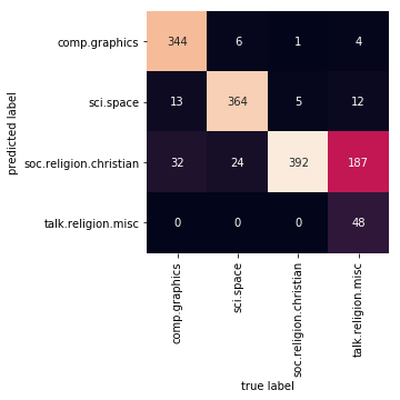
Evidently, even this very simple classifier can successfully separate space talk from computer talk, but it gets confused between talk about religion and talk about Christianity. This is perhaps an expected area of confusion!

The very cool thing here is that we now have the tools to determine the category for any string, using the predict() method of this pipeline. Here’s a quick utility function that will return the prediction for a single string:

predict_category('discussing islam vs atheism')

'soc.religion.christian'

predict_category('determining the screen resolution')

'comp.graphics'

predict_category('sending a payload to the ISS')

'sci.space'

When to Use Naive Bayes

Because naive Bayesian classifiers make such stringent assumptions about data, they will generally not perform as well as a more complicated model. That said, they have several advantages:

• They are extremely fast for both training and prediction

• They provide straightforward probabilistic prediction

• They are often very easily interpretable

• They have very few (if any) tunable parameters

These advantages mean a naive Bayesian classifier is often a good choice as an initial baseline classification.