%run ../initscript.py
HTML("""
<div id="popup" style="padding-bottom:5px; display:none;">
    <div>Enter Password:</div>
    <input id="password" type="password"/>
    <button onclick="done()" style="border-radius: 12px;">Submit</button>
</div>
<button onclick="unlock()" style="border-radius: 12px;">Unclock</button>
<a href="#" onclick="code_toggle(this); return false;">show code</a>
""")

Enter Password:

Submit

Unclock show code

%run loadmlfuncs.py

df_book_part1 = pd.read_csv(dataurl+'book_train.csv', header=0, index_col='customer')
df_book_part2 = pd.read_csv(dataurl+'book_validation.csv', header=0, index_col='customer')

toggle()

show code

Logistic Regression

Logistic regression is a popular method for classifying individuals (although we call it regression), given the values of a set of explanatory variables. It estimates the probability that an individual is in a particular category. We will demonstrate the method by considering a book club case.

Book Club

In a book club, a new title, “The Art History of Florence”, is ready for release. The book club has sent promotion mails to a sample of customers from its customer base in two different times. Each time it randomly select 1000 customers.

df_book_part1.head()

	month	art_book	purchased
customer
1	24	0	0
2	16	0	0
3	15	0	0
4	22	0	0
5	15	0	1

df_book_part2.head()

	month	art_book	purchased
customer
1001	30	0	0
1002	12	0	0
1003	18	0	0
1004	27	1	0
1005	4	1	0

Book club has collected several variables for all 2000 customers as follows:

• month: months to the customer’s last purchase when promotion mail is sent

• art_book: number of art books the customer purchased before

• purchased: if s/he paid for the new title “The Art History of Florence”

It costs the book club $1 for sending a mail and generates $7 profit for selling the book. After two promotions, an analyst in the book club realizes that the store actually lost money in both promotions.

def calc_profit(df):
    mail_cost = 1
    selling_profit = 7
    profit = df.purchased.sum() * 7 - df.month.count()*mail_cost
    return profit

print('net profit for the 1st promotion:', calc_profit(df_book_part1))
print('net profit for the 2nd promotion:', calc_profit(df_book_part2))

net profit for the 1st promotion: -418
net profit for the 2nd promotion: -433

The manager believes that the book club should build a predictive model to predict each customer’s probability of purchasing, and then send out promotion mail only if such a probability is high enough.

• can we derive a prediction model after collecting the data from the first promotion?

• can this prediction model improve the second promotion?

We expect this prediction model

• uses month and art_book to predict purchased

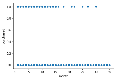
which suggests a regression equation purchased \(\sim\) month \(+\) art_book. However, the \(y\) variable purchased is either 0 or 1, and a scatter plot between purchased and month (\(y\) vs \(x\)) shows as follows

df_book_part1.plot.scatter(x='month', y='purchased')
plt.show()

The graph is against many linear regression assumptions:

• there is no linear relationship between independent and dependent variables.

• error term is probably not normally distributed.

The Model

Instead of using the binary variable (purchased or not), we may consider purchasing probability \(p\) as dependent variable in a regression equation such as

\begin{align} p &= \beta_0 + \beta_1 \times \text{month} + \beta_2 \times \text{art_book} \end{align}

Although \(p\) is continuous, we still cannot run a linear regression on \(p\) because it is bounded in range \([0,1]\). In linear regression, the dependent variable should be able to take any value in range \([-\infty, +\infty]\).

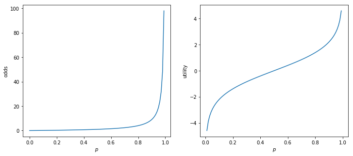
We introduce odds and utility

\begin{align} \text{odds} &= \frac{p}{1-p} \nonumber \\ \text{utility} &= \log(\text{odds}) \nonumber \\ \end{align}

Note that utility is in \([-\infty, +\infty]\). Now a regression equation can be used

\begin{align} \text{utility} &= \beta_0 + \beta_1 \times \text{month} + \beta_2 \times \text{art_book} \end{align}

p = np.linspace(0,1,100)
odds = p / (1-p)
utility = np.log(odds)

plt.subplots(1, 2, figsize=(12,5))
plt.subplot(1, 2, 1)
plt.plot(p, odds)
plt.xlabel('$p$')
plt.ylabel('odds')

plt.subplot(1, 2, 2)
plt.plot(p, utility)
plt.xlabel('$p$')
plt.ylabel('utility')

plt.show()
toggle()

show code

In practice, we can simply use a typical type of regression, logistic regression, with binary dependent variable. Statistical tools will perform all the transformation for us. In python, we can use either statmodels which provides statistical summary or sklearn package.

from statsmodels.api import add_constant
from statsmodels.formula.api import Logit
X = add_constant(df_book_part1[['month','art_book']])
y = df_book_part1['purchased']
model = Logit(y, X)
model.fit().summary()

Optimization terminated successfully.
         Current function value: 0.251705
         Iterations 7

Logit Regression Results

Dep. Variable:	purchased	No. Observations:	999
Model:	Logit	Df Residuals:	996
Method:	MLE	Df Model:	2
Date:	Mon, 29 Jul 2019	Pseudo R-squ.:	0.1206
Time:	20:41:18	Log-Likelihood:	-251.45
converged:	True	LL-Null:	-285.95
		LLR p-value:	1.044e-15

	coef	std err	z	P>|z|	[0.025	0.975]
const	-2.2262	0.239	-9.316	0.000	-2.695	-1.758
month	-0.0706	0.019	-3.670	0.000	-0.108	-0.033
art_book	0.9888	0.135	7.343	0.000	0.725	1.253

The signs of the coefficients indicate whether the probability of purchasing the book increases or decreases when these variables increases. For example, the probability of purchasing the book decrease as month increase (because of its minus sign) and increase as art_book increase (because of its plus sign).

However, you have to use caution when interpreting the magnitudes of the coefficients. For example, the absolute value of coefficient of month is smaller than art_book because month generally have larger values than art_book.

The value \(\exp\)(coefficient) is more interpretable. For example, if art_book increases 1, the odds of purchasing the book increase by a factor about \(\exp(0.9888)\). So, you should be on the lookout for values well above or below 1.

from sklearn import linear_model

X = df_book_part1[['month','art_book']]
y = df_book_part1['purchased']

clf = linear_model.LogisticRegression(C=1e5, solver='lbfgs')
clf.fit(X, y)
print('intercept=', clf.intercept_, '\ncoefficient =', clf.coef_)

intercept= [-2.22621349]
coefficient = [[-0.07061966  0.98880806]]

Validation

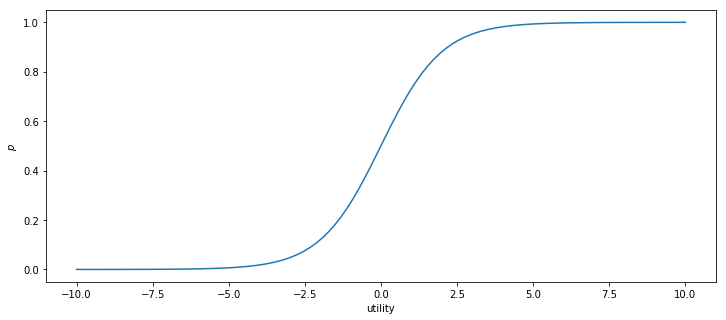
After we have obtained \(\beta_0, \beta_1\) and \(\beta_2\), we can use equation \((2)\) for our validation data to evaluate its utility. Then, the probability can be derived by

\begin{align} p = \frac{\exp(\text{utility})}{1+\exp(\text{utility})} \nonumber \end{align}

utility = np.linspace(-10,10,100)
p = np.exp(utility) / (1 + np.exp(utility))

plt.subplots(1, 1, figsize=(12,5))
plt.plot(utility, p)
plt.xlabel('utility')
plt.ylabel('$p$')
plt.show()
toggle()

show code

In general, our decision can be made based on a threshold value 0.5. That is, if the probability that a customer may purchase the book is greater than 0.5, we send a mail.

However, in the book club case, it has a simple break-even point where the cost-profit ratio is \(1/7\). Therefore, our strategy can be designed based on this ratio as follows. If the probability that a customer may purchase the book is greater than \(1/7\), we send a mail, otherwise we do not.

We prefer to use sklearn because it provides capability to predict the probability directly.

df_book_part2['purchase_prob'] = clf.predict_proba(df_book_part2[['month','art_book']])[:,1]
df_book_part2['send'] = df_book_part2['purchase_prob'] > 1/7
df_book_part2.head()

	month	art_book	purchased	purchase_prob	send
customer
1001	30	0	0	0.012808	False
1002	12	0	0	0.044207	False
1003	18	0	0	0.029387	False
1004	27	1	0	0.041323	False
1005	4	1	0	0.179479	True

num_mail_send = df_book_part2[df_book_part2['send']].shape[0]
num_purchased = df_book_part2[df_book_part2['send'] & df_book_part2['purchased'] == 1].shape[0]
profit = num_purchased * 7 - num_mail_send
print('Based on our prediction model, we should send {} mails.'.format(num_mail_send))
print('We would expect receiving {} orders and our profit is ${}.'.format(num_purchased, profit))
toggle()

Based on our prediction model, we should send 128 mails.
We would expect receiving 38 orders and our profit is $138.

show code